Deep Learning for Brain Volumetry in Contrast-Enhanced MRI: Methods, Validation, and Clinical Applications
This article explores the application of deep learning (DL) for brain volumetry using contrast-enhanced MRI (CE-MRI), a significant area of interest for neuroscience research and drug development.
Deep Learning for Brain Volumetry in Contrast-Enhanced MRI: Methods, Validation, and Clinical Applications
Abstract
This article explores the application of deep learning (DL) for brain volumetry using contrast-enhanced MRI (CE-MRI), a significant area of interest for neuroscience research and drug development. It covers the foundational principles of extracting volumetric data from CE-MRI, a resource often underutilized due to technical heterogeneity. We delve into specific methodological approaches, including segmentation tools like SynthSeg+ and novel architectures for predicting contrast-equivalent information from non-contrast scans. The content addresses critical troubleshooting aspects, such as mitigating hallucinations and false positives in DL models, and performance optimization. Finally, it provides a comprehensive validation and comparative analysis of different DL techniques against traditional methods and ground truth, evaluating their reliability and clinical applicability. This synthesis aims to equip researchers and drug development professionals with a clear understanding of the current landscape, challenges, and future potential of DL-based brain volumetry.
The Foundation of Deep Learning Volumetry in Contrast-Enhanced MRI
Quantitative Evidence of Underutilization
Clinical guidelines increasingly support contrast-enhanced magnetic resonance imaging (CE-MRI) for various indications, but its adoption in clinical and research practice remains inconsistent. The data below summarize the key evidence of this underutilization.
Table 1: Evidence of CE-MRI Underutilization in Medical Practice
| Evidence Aspect | Quantitative Finding | Context & Source |
|---|---|---|
| Supplemental Breast MRI in High-Risk Women | Only 6.6% (158/2403) of high-lifetime-risk women received supplemental breast MRI screening within a 2-year window despite 43.9% attending a facility with on-site availability [1]. | Cross-sectional study of 422,406 screening mammograms across 86 U.S. facilities (2018 data) [1]. |
| Geographic Variability of CMR Access | 16 CMR centers per million U.S. Medicare beneficiaries, with state density ranging from 52.6 (MN, highest) to 4.4 (ME, lowest) per million [2]. | U.S. national analysis based on 2018 Medicare claims data [2]. |
| High-Volume Center Proficiency | 53% (59/112) of surveyed CMR centers were high-volume (>500 scans/year) in 2019, with these centers averaging 19 years of experience, compared to 3.5 years for low-volume centers [2]. | Society for Cardiovascular Magnetic Resonance (SCMR) survey data from 2017-2019 [2]. |
Core Principles and Protocol for DCE-MRI
Dynamic Contrast-Enhanced MRI (DCE-MRI) is a key CE-MRI technique that enables the quantitative assessment of tissue vascularity, permeability, and blood flow by tracking the kinetics of an injected contrast agent [3] [4].
Fundamental Physics and Mechanism of Action
- Contrast Agent Effect: Gadolinium-based contrast agents (GBCAs) are paramagnetic. They shorten the T1 (longitudinal) relaxation time of nearby water protons, resulting in increased signal intensity on T1-weighted images [5] [3].
- Blood-Brain Barrier (BBB) Leakage: In a healthy brain, the intact BBB prevents GBCAs from leaking into the brain tissue. In many neurological disorders, BBB disruption allows GBCAs to extravasate into the extravascular extracellular space (EES), causing visible enhancement and enabling permeability quantification [4].
Detailed DCE-MRI Acquisition Protocol
The following workflow outlines the standard procedure for acquiring DCE-MRI data.
DCE-MRI Data Analysis and Pharmacokinetic Modeling
Quantitative analysis uses pharmacokinetic (PK) models to convert signal intensity changes into physiological parameters [3] [4].
Table 2: Key Pharmacokinetic Parameters in DCE-MRI
| Parameter | Physiological Meaning | Interpretation |
|---|---|---|
| Ktrans (volume transfer constant) | Permeability-surface area product per unit volume of tissue [4]. | High Ktrans indicates increased vascular permeability or blood flow, common in tumors with angiogenesis [4]. |
| Ve (extravascular extracellular volume) | Fractional volume of the extravascular extracellular space (EES) [4]. | Represents the fractional volume of the EES [4]. |
| kep (rate constant) | Flux rate constant between EES and blood plasma (kep = Ktrans/Ve) [4]. | Reflects the washout rate of the contrast agent from the EES back to the bloodstream [4]. |
| Vp (plasma volume) | Fractional blood plasma volume [4]. | Represents the fractional volume of blood plasma in the tissue [4]. |
Application Notes & Experimental Protocols
Application in Preclinical Drug Development
CE-MRI, particularly DCE-MRI, provides objective, quantitative biomarkers crucial for central nervous system (CNS) drug development [6].
- Phase I Trials: DCE-MRI can demonstrate CNS penetration and confirm target engagement for drugs that may not be amenable to positron emission tomography (PET) imaging [6].
- Phase II/III Trials: The technique can differentiate objective measures of drug efficacy from placebo response, a major challenge in CNS trials. It helps identify responders versus non-responders and can provide insights into disease modification [6].
Sample Experimental Protocol: Evaluating Anti-Angiogenic Therapy in Glioblastoma
- Subject Preparation: Animal model or human patient with a confirmed glioma.
- Baseline DCE-MRI: Perform DCE-MRI as detailed in Section 2.2.
- Therapy Administration: Administer the anti-angiogenic drug candidate.
- Follow-up DCE-MRI: Repeat the DCE-MRI at predetermined time points (e.g., 2 weeks, 4 weeks).
- Data Analysis: Calculate Ktrans, Ve, and Vp maps. A successful therapeutic response is indicated by a significant decrease in Ktrans values in the tumor region, reflecting reduced vascular permeability and angiogenesis [4].
Deep Learning for Contrast Enhancement and Volumetry
Emerging deep learning (DL) techniques aim to overcome CE-MRI limitations, such as the need for gadolinium and long acquisition times [7] [8].
- Gadolinium-Free Contrast Mapping: DL models can now generate synthetic contrast-enhanced maps or estimate cerebral blood volume (CBV) from a single, non-contrast T1-weighted scan, eliminating patient risk from gadolinium administration [7].
- Rapid, Automated Volumetry: DL enables fully automatic segmentation of brain volumes from MRI, even in challenging preclinical settings. This dramatically reduces acquisition times (e.g., from >12 minutes to ~4.3 minutes for mouse brain volumetry) and provides robust, high-throughput analysis for longitudinal studies [8].
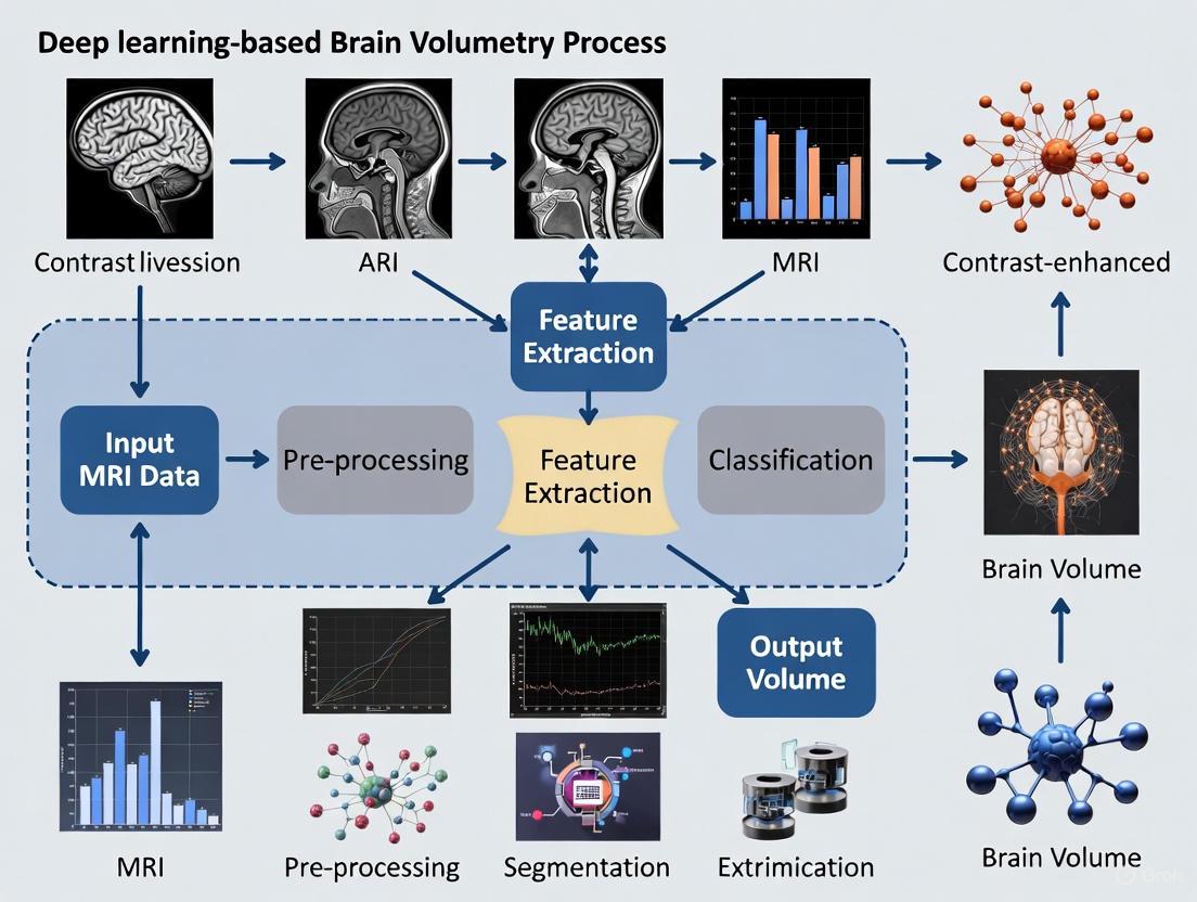
Sample Experimental Protocol: Deep Learning-Based Brain Volumetry in Neurodegeneration
- Data Acquisition: Acquire high-resolution T2-weighted images (or other modalities) according to the optimized, fast protocol enabled by DL reconstruction [8].
- Preprocessing: Perform skull-stripping and image registration to a standard atlas space using automated DL tools [8].
- Semantic Segmentation: Input preprocessed images into a trained neural network (e.g., 3D CNN, Mamba-based model) for voxel-wise classification [7] [8].
- Volumetric Calculation: Compute the total brain and sub-region (e.g., hippocampus, caudate putamen) volumes from the segmentation masks [8].
- Longitudinal Analysis: Track volume changes over time to assess disease progression or treatment effects in models of Alzheimer's disease, multiple sclerosis, etc. [8].
The diagram below illustrates this integrated deep learning workflow.
The Scientist's Toolkit: Research Reagent Solutions
Table 3: Essential Materials and Reagents for CE-MRI Research
| Item | Function/Description | Key Considerations |
|---|---|---|
| Gadolinium-Based Contrast Agent (GBCA) | Pharmaceutical that shortens T1 relaxation time to create image contrast [5] [3]. | Choose between linear/macrocyclic and ionic/non-ionic types based on conditional stability and NSF risk profile [5]. Macrocyclic agents generally have higher stability [5]. |
| Power Injector | Ensures a precise, rapid, and reproducible intravenous bolus injection of the GBCA. | Critical for consistent DCE-MRI data acquisition and reliable pharmacokinetic modeling [3] [4]. |
| Pharmacokinetic Modeling Software | Software that fits PK models (e.g., Extended Toft, Patlak) to dynamic data to compute parameters like Ktrans and Ve [4]. | Model selection is crucial; the Patlak model is often recommended for subtle BBB leakage in neurodegeneration [4]. |
| Deep Learning Segmentation Framework | A trained neural network (e.g., 3D U-Net) for automated, voxel-wise labeling of brain anatomical regions [8]. | Dramatically increases analysis throughput and reproducibility for brain volumetry studies compared to manual segmentation [8]. |
| Reference Region Atlas | A standardized template with pre-defined anatomical boundaries for different brain regions. | Essential for registration-based segmentation and for validating the accuracy of automated DL segmentation methods [8]. |
Technical heterogeneity in Magnetic Resonance Imaging (MRI) presents a fundamental challenge for the development and deployment of robust deep learning (DL) tools in neuroscience research and drug development. Variability across scanners, vendors, acquisition protocols, and sites introduces confounding noise that can obscure biological signals, compromise biomarker validity, and reduce the generalizability of predictive models. For DL-based brain volumetry and contrast-enhanced MRI research, this heterogeneity directly impacts measurement reproducibility, potentially leading to inaccurate assessment of therapeutic efficacy in clinical trials. The "Cycle of Quality" framework emphasizes that addressing these technical confounds is not merely a preprocessing step but an essential, integrated process spanning from acquisition to analysis [9]. This Application Note provides detailed protocols and analytical frameworks to identify, quantify, and mitigate these sources of variation, enabling more reliable and reproducible DL-driven biomarkers.
Technical heterogeneity manifests across multiple dimensions of the MRI acquisition pipeline. The tables below summarize key sources of variability and their documented impact on quantitative outcomes.
Table 1: Primary Sources of Technical Heterogeneity in MRI Acquisition
| Source Category | Specific Parameters | Impact on Quantitative MRI |
|---|---|---|
| Hardware | Scanner Manufacturer & Model, Magnetic Field Strength (e.g., 3T vs. 7T), RF Coil Type (Conventional vs. Cryogenic) | Affects fundamental signal-to-noise ratio (SNR), spatial resolution, and geometric distortion [8] [9]. |
| Sequence Protocol | Pulse Sequence Type (SE, GRE, RARE), Timing Parameters (TR, TE), Flip Angle, Voxel Dimensions | Directly influences image contrast, SNR, and the relationship between signal intensity and underlying tissue properties (e.g., T1, T2) [10]. |
| Reconstruction & Processing | Reconstruction Algorithm, Use of Parallel Imaging, Post-processing Filters, Vendor-specific Software | Introduces variation in noise texture, sharpness, and can create artifacts that may be learned by DL models as false features [9]. |
| Phantom & Calibration | Phantom Composition, Calibration Schedule, Quality Control Procedures | Leads to scanner-specific drifts in quantitative values over time, affecting longitudinal study reliability [9]. |
Table 2: Documented Performance of Deep Learning Models Under Heterogeneous Conditions
| DL Application | Model Input/Strategy | Key Metric | Performance Outcome | Context of Heterogeneity |
|---|---|---|---|---|
| CBV Map Synthesis [11] | Single-modal non-contrast scan | N/A (Qualitative Validation) | Identified functional abnormalities in aging and Alzheimer's disease brains. | Trained on quantitative steady-state contrast-enhanced MRI to overcome variability in radiological scans. |
| Mouse Brain Volumetry [8] | T2-weighted images (4.3 min acquisition) | Reproducibility in Healthy Mice | Reliable quantification of hippocampus, caudate putamen, and cerebellum volumes. | High spatial resolution (78x78x250 μm³) challenge at 7T; DL enabled fast, consistent segmentation. |
| Gadolinium-Free CE-MRI [12] | NC-MRI (T2w, DWI, Pre-contrast T1w) | Sensitivity/Specificity for HCC | 0.866 / 0.922 (vs. 0.899 / 0.925 for conventional CE-MRI) | Model generalized across three institutions, synthesizing multiple contrast phases from non-contrast inputs. |
| Synthetic Post-Contrast T1 [11] | Multi-parametric MRI (T1w, T2w, FLAIR, DWI, SWI) | PSNR / SSIM | 22.967 ± 1.162 / 0.872 ± 0.031 (BayesUNet) | Comprehensive input protocol designed to capture diverse tissue contrasts for robust synthesis. |
Experimental Protocols for Harmonization and Validation
Protocol 1: Prospective Multi-Scanner Harmonization
This protocol outlines a framework for standardizing acquisition across multiple sites or scanners, a critical step for multi-center clinical trials.
A. Pre-Study Calibration and Phantom Imaging
- Objective: To establish a baseline for signal and geometric fidelity across all scanners in the network.
- Materials: Standardized imaging phantom (e.g., ADNI phantom or custom design with known relaxation properties and geometric features).
- Methodology:
- Protocol Translation: Convert the core research sequence (e.g., T1-weighted 3D MPRAGE) into vendor-specific implementations (e.g., "BRAVO" on GE, "MPRAGE" on Siemens, "3D T1 FFE" on Philips) while keeping core parameters (TR, TE, TI, resolution) as consistent as possible.
- Phantom Imaging: Perform weekly phantom scans on each participating scanner using the translated protocols over a one-month stability period.
- Metric Extraction: Analyze phantom data to quantify:
- Signal-to-Fluctuation-Noise Ratio (SFNR): For temporal stability.
- Geometric Distortion: Measure known distances in the phantom versus acquired images.
- Intensity Uniformity: Profile signal variation across the field-of-view.
- Validation: Inter-scanner coefficient of variation (CoV) for all extracted metrics should be <5% before proceeding to in-vivo imaging.
B. In-Vivo Traveling Subject Study
- Objective: To quantify inter-scanner variability on biological measurements.
- Methodology:
- Recruit a small cohort (n=3-5) of "traveling subjects" who can be scanned on all participating scanners within a short time window (e.g., 2 weeks).
- Acquire the full imaging protocol on each subject at each site.
- Process data through a centralized, standardized pipeline for brain extraction, tissue segmentation (GM, WM, CSF), and regional volumetry (e.g., of the hippocampus).
- Analysis: Calculate the intra-class correlation coefficient (ICC) and CoV for key volumetric outputs (e.g., total brain volume, hippocampal volume) across scanners. An ICC > 0.9 is considered excellent for multi-center studies.
Protocol 2: Retrospective Harmonization using Deep Learning
For existing datasets where prospective harmonization was not feasible, this protocol uses DL to mitigate site effects.
A. Data Preprocessing and Feature Extraction
- Objective: To prepare heterogeneous data for harmonization.
- Methodology:
- Standardized Preprocessing: Apply a consistent pipeline to all datasets, including N4 bias field correction, intensity-based brain extraction, and affine registration to a standard template (e.g., MNI space).
- Feature Extraction: For volumetry tasks, use a pre-trained DL segmentation model (e.g., a U-Net variant) to generate regional volume maps. For intensity-based tasks, extract features from the normalized native space images.
B. Harmonization Model Training (ComBat-GAN)
- Objective: To remove technical site/scanner effects while preserving biological variance.
- Methodology:
- Apply Statistical Harmonization: Use a validated method like ComBat (or its Bayesian extension) to remove site effects from the extracted features or volumetric maps. This model adjusts for location and scale (mean and variance) differences between sites.
- Train Generative Adversarial Network (GAN): To synthesize harmonized images directly, train a CycleGAN or similar architecture. The model learns a mapping between images from different sites, effectively translating a scan from "Scanner A style" to "Scanner B style" or to a common harmonized "style".
- Input: Paired (or unpaired) patches from different scanners/sites.
- Generator Loss: Combination of adversarial loss and cycle-consistency loss.
- Output: Harmonized image patches that retain subject-specific biology but exhibit consistent image properties.
- Validation: Demonstrate that a DL classifier can no longer predict the scanner source from the harmonized data with accuracy above chance, while performance on a biological task (e.g., patient vs. control classification) is maintained or improved.
Visualization of Workflows and Logical Frameworks
The Quality Cycle in MRI Research
This diagram illustrates the integrated, cyclical process required to achieve and maintain quality in multi-site MRI research, from initial concept to disseminated results.
Technical Validation Pathway for DL Volumetry
This workflow outlines the specific steps for technically validating a deep learning brain volumetry pipeline against a ground truth reference method.
The Scientist's Toolkit: Key Research Reagents & Materials
Table 3: Essential Resources for Managing MRI Heterogeneity in DL Research
| Tool Category | Specific Tool / Reagent | Function & Utility | Key Considerations |
|---|---|---|---|
| Reference Phantoms | ADNI Phantom; Custom QMRI Phantoms | Provides a stable ground truth for scanner calibration and longitudinal monitoring of scanner drift [9]. | Phantoms should mimic tissue relaxation properties (T1, T2) and be MRI-safe for the long term. |
| Standardized Atlases | Mouse Brain ATLAS (e.g., from [8]); Human Brain Templates (MNI, ICBM) | Serves as a common coordinate system for spatial normalization and inter-subject registration, crucial for comparative analysis. | Atlas choice should be appropriate for the study population (e.g., age, species, disease). |
| Harmonization Software | ComBat (and its variants); Pulseq [9] | ComBat: Statistically removes batch effects from extracted features. Pulseq: Enables vendor-neutral, reproducible sequence programming. | ComBat requires careful modeling to avoid removing biological signal. Pulseq needs vendor approval/installation. |
| Deep Learning Frameworks | U-Net Architectures; Stable Diffusion Models [12]; Generative Adversarial Networks (GANs) | U-Net: Gold-standard for segmentation tasks. GANs: Used for data augmentation [14] and image harmonization. Stable Diffusion: Can synthesize contrast-enhanced images from non-contrast inputs [12]. | Models must be trained on diverse, well-characterized datasets to ensure generalizability. |
| Validation Datasets | Traveling Human / Mouse Data; Multi-site Public Databases (e.g., ADNI) | Provides the "ground truth" for inter-scanner variability, allowing for quantitative assessment of harmonization methods. | Traveling subject studies are the gold standard but are resource-intensive to execute. |
Technical heterogeneity in MRI is a formidable but manageable challenge. Through the systematic application of prospective harmonization protocols, robust retrospective data cleaning techniques, and the strategic use of deep learning models designed for domain adaptation, researchers can extract reliable, reproducible quantitative biomarkers. The frameworks and toolkits provided here offer a concrete pathway for achieving this goal. As the field moves forward, embracing the "Cycle of Quality" and embedding these practices into the core of research and drug development workflows will be paramount for translating promising DL-based imaging biomarkers into validated tools for clinical trials and patient care.
Brain morphometry, the quantitative study of brain structure, is a critical neuroimaging biomarker for diagnosing and monitoring neurological and neurodegenerative diseases. In clinical practice, a significant portion of magnetic resonance imaging (MRI) examinations include contrast-enhanced (CE-MR) sequences, primarily for improving pathological lesion detection. However, the reliability of CE-MR scans for quantitative morphometric analysis has remained uncertain due to potential signal alteration from gadolinium-based contrast agents. This application note examines the physics basis underlying this question and demonstrates, through quantitative evidence and protocol details, that advanced deep learning methods now enable reliable morphometry from CE-MR scans, thereby expanding the potential dataset for neuroscience research and drug development.
Quantitative Evidence: Comparative Performance of Segmentation Tools
Table 1: Reliability of Volumetric Measurements Between CE-MR and NC-MR Scans [15] [16]
| Brain Structure | Segmentation Tool | Intraclass Correlation Coefficient (ICC) | Notes |
|---|---|---|---|
| Most Brain Regions | SynthSeg+ | > 0.90 | Demonstrates high reliability for most structures |
| Larger Brain Structures | SynthSeg+ | > 0.94 | Even stronger agreement in larger volumes |
| Brain Stem | SynthSeg+ | > 0.90 (lowest, but robust) | Shows the lowest, yet still high, correlation |
| Global Gray Matter | CAT12 | ICC = 0.87 | Good agreement |
| Hippocampus | CAT12 | ICC = 0.57 | Poor agreement |
| Amygdala | CAT12 | ICC = 0.45 | Poor agreement |
| CSF & Ventricular Volumes | SynthSeg+ | Discrepancies noted | Systematic differences observed |
Table 2: Scan-Rescan Reliability of Volumetric Tools Across Multiple Scanners [17]
| Software Solution | Median CV for GM Volume | Median CV for WM Volume | Median CV for Total Brain Volume | Performance Category |
|---|---|---|---|---|
| AssemblyNet | < 0.2% | < 0.2% | 0.09% | High Reliability |
| AIRAscore | < 0.2% | < 0.2% | 0.09% | High Reliability |
| FastSurfer | > 0.2% | < 0.2% | > 0.2% | Moderate Reliability |
| FreeSurfer | > 0.2% | > 0.2% | > 0.2% | Moderate Reliability |
| SPM12 | > 0.2% | > 0.2% | > 0.2% | Moderate Reliability |
| syngo.via | > 0.2% | > 0.2% | > 0.2% | Moderate Reliability |
| Vol2Brain | > 0.2% | > 0.2% | > 0.2% | Moderate Reliability |
The quantitative evidence confirms that with appropriate tool selection, CE-MR scans can reliably support morphometry. The deep learning-based tool SynthSeg+ demonstrates exceptionally high consistency between CE-MR and non-contrast MR (NC-MR) scans, with Intraclass Correlation Coefficients (ICCs) exceeding 0.90 for most brain structures [15] [16]. In contrast, traditional tools like CAT12 show inconsistent performance, with poor reliability for smaller structures like the hippocampus and amygdala (ICC < 0.60) [15] [16].
For longitudinal studies, scan-rescan reliability is paramount. Recent multi-scanner assessments reveal that modern AI-based tools AssemblyNet and AIRAscore achieve superior precision, with median coefficients of variation (CV) for gray matter (GM), white matter (WM), and total brain volume all below 0.2% [17]. The study found that the choice of software has a stronger effect on measurement variance than the scanner hardware itself [17].
Experimental Protocols for Validating CE-MR Morphometry
Core Experimental Workflow
The following diagram illustrates the key steps for a validation experiment comparing morphometric measurements from CE-MR and NC-MR scans.
Detailed Methodology
1. Participant Cohort & Image Acquisition:
- Cohort: A typical study should include clinically normal participants across a wide age range (e.g., 21-73 years) to assess generalizability. A sample size of approximately 60 subjects provides robust power for reliability analysis [15] [16].
- MRI Protocol: Acquire paired T1-weighted NC-MR and CE-MR scans for each participant in a single session. For CE-MR, use a standard gadolinium-based contrast agent (e.g., Gd-DTPA) with a dose of 0.25 mL/kg, injected via cubital vein at 1 mL/s, followed by a 3-minute delay before scanning [18]. Ensure consistent sequence parameters (e.g., 3D FFE, matrix=256×256, 1mm isotropic voxels) between the two scan types [18].
2. Image Preprocessing Pipeline:
- Resampling: Standardize the spatial resolution of all MRI scans to a uniform isotropic voxel size (e.g., 0.833 mm³) to minimize variability [18].
- Skull Stripping: Remove non-brain tissues using an advanced, robust tool like SynthStrip to reduce computational overhead and focus analysis on brain tissue [18].
- Intensity Normalization: Apply Z-score normalization to standardize voxel intensities across subjects, mitigating inter-scanner and inter-subject variability [18].
- Quality Control: Implement an automated verification step to ensure alignment between MRI scans and segmentation masks. Visually inspect intensity histograms to ensure consistency [18].
3. Segmentation and Volumetric Analysis:
- Tool Selection: Employ a combination of segmentation tools for comparison, prioritizing deep learning-based methods (e.g., SynthSeg+, AssemblyNet) known for their robustness to contrast variation [15] [16] [17].
- Execution: Process all NC-MR and CE-MR scans through the selected pipelines to extract volumetric measurements for key brain structures (global GM, WM, ventricles, and subcortical nuclei).
4. Statistical Validation:
- Reliability Analysis: Calculate Intraclass Correlation Coefficients (ICCs) between measurements from CE-MR and NC-MR scans for all segmented structures. ICC values > 0.90 are considered indicative of high reliability [15] [16].
- Scan-Rescan Variability: For studies across multiple scanners, calculate the percentage Coefficient of Variation (%CV) to assess the precision of each software tool. A lower CV indicates higher reliability [17].
- Bland-Altman Plots: Use these plots to visualize the agreement between CE-MR and NC-MR measurements and identify any systematic biases [17].
- Downstream Validation: Build age prediction models or correlate volumetric measures with clinical severity scores (e.g., WAB-R for aphasia) using both CE-MR and NC-MR-derived data. Comparable model performance further validates the utility of CE-MR scans [15] [19].
The Scientist's Toolkit: Essential Research Reagents & Software
Table 3: Key Software Solutions for Deep Learning-Based Morphometry
| Tool Name | Type/Function | Key Application in CE-MR Research |
|---|---|---|
| SynthSeg+ | Deep learning-based segmentation tool | Robust brain volume segmentation from both CE-MR and NC-MR scans; high ICC reliability [15] [16]. |
| 3D U-Net (with ResNet-34) | Convolutional Neural Network architecture | Volumetric medical image segmentation (e.g., for brain metastases); uses patch-based training [18]. |
| AssemblyNet | AI-based volumetric tool | Provides high scan-rescan reliability (CV < 0.2%) for GM, WM, and total brain volume [17]. |
| AIRAscore | Certified medical device software | Demonstrates high precision in longitudinal volumetry (CV < 0.2%) across different scanners [17]. |
| FreeSurfer | Established morphometry pipeline | Widely used for generating silver-standard ground truth; provides comprehensive cortical and subcortical metrics [20]. |
| CAT12 | SPM-based segmentation toolbox | Traditional tool for voxel-based morphometry; shows inconsistent performance on CE-MR scans [15] [16]. |
The physics basis for utilizing CE-MR scans in morphometry is robust when supported by modern deep learning methodologies. Evidence confirms that advanced tools like SynthSeg+, AssemblyNet, and AIRAscore can mitigate the effects of contrast agent, enabling reliable volumetric measurements from clinically acquired CE-MR images. This breakthrough significantly expands the potential pool of data for large-scale neuroimaging research and drug development trials by allowing the quantitative use of vast existing clinical datasets. For conclusive results, researchers must adhere to standardized protocols, prioritize deep learning-based segmentation tools, and maintain consistency in scanner-software combinations throughout their studies. Future work will focus on refining models to reduce remaining discrepancies in CSF and ventricular volumes and further validating these approaches in specific patient populations.
Deep Learning's Role in Learning Non-Linear Mappings for Volumetry
Deep learning (DL) has emerged as a transformative technology for brain volumetry, primarily through its capacity to learn complex, non-linear mappings from medical images to quantitative volumetric outputs. These mappings enable the direct estimation of brain structure volumes from input data, bypassing traditional intermediate steps that often require manual intervention or simplified linear models. The non-linear nature of deep neural networks allows them to capture intricate relationships within image data that conventional algorithms might miss, leading to more accurate and robust volumetry across diverse patient populations and imaging protocols. This capability is particularly valuable in neurodegeneration research and drug development, where precise measurement of brain structures serves as a critical biomarker for disease progression and therapeutic efficacy [21].
DL models learn these mappings through a training process where network parameters are iteratively adjusted to minimize the difference between predicted volumetric outputs and known ground-truth labels. This process allows the models to identify and leverage subtle patterns in the imaging data, such as textural variations and shape descriptors, that correlate with anatomical boundaries. For clinical researchers and drug development professionals, this technology offers two significant advantages: the automation of labor-intensive manual segmentation processes and the ability to extract additional quantitative information from standard clinical scans that would otherwise require specialized acquisition protocols or contrast agents [11] [22].
Key Applications and Experimental Data
Table 1: Performance Metrics of Deep Learning Volumetry Applications
| Application Area | Key Metric | Performance Value | Reference/Model |
|---|---|---|---|
| MRI Acceleration | Scan Time Reduction | 2x faster (1 min 10 s vs. 4 min 59 s) | DL-Speed [23] |
| MRI Acceleration | Total GM Volume Correlation | r = 0.99 (p < 0.001) | DL-Speed [23] |
| MRI Acceleration | Hippocampal Occupancy Score | 0.68 ± 0.17 (no significant difference) | SubtleMR + NeuroQuant [22] |
| Contrast-Free CBV Mapping | Peak Signal-to-Noise Ratio | 22.967 ± 1.162 | BayesUNet [11] |
| Contrast-Free CBV Mapping | Structural Similarity Index | 0.872 ± 0.031 | BayesUNet [11] |
| DCE-MRI Analysis | Computational Time Reduction | 17 s vs. 15 min | CNNCON [24] |
| DCE-MRI Analysis | Ktrans MAE | (111 ± 70) × 10⁻⁵ min⁻¹ | CNNCON [24] |
| CT Volumetry | Dementia vs Control Differentiation | High accuracy (comparable to MRI) | U-Net [25] |
Protocol Acceleration and Contrast Agent Elimination
A primary application of non-linear mapping in volumetry is the significant acceleration of MRI acquisition protocols. Watanabe et al. demonstrated that a deep learning-based reconstruction technique (DL-Speed) enables approximately one-minute 3D T1-weighted imaging, reducing scan times from nearly five minutes to just over one minute while preserving quantitative integrity for morphometric analysis [23]. This acceleration directly addresses patient motion artifacts, with the DL-Speed protocol showing significantly reduced head motion (Total Vector Change: 52.3 ± 9.4 mm vs. 140.4 ± 32.8 mm, p < 0.001) while maintaining acceptable image quality for cortical thickness and gray matter volume measurements [23]. Independent validation of FDA-cleared DL software (SubtleMR) confirmed that 2x faster scan times produce hippocampal occupancy scores and volumetric measures with no statistical difference from standard protocols, demonstrating strong generalizability across five different 3T scanners [22].
Beyond acceleration, DL has enabled the complete elimination of gadolinium-based contrast agents (GBCAs) from certain functional imaging protocols. Liu et al. developed a deep learning model that maps single-modal non-contrast MRI scans to synthetic cerebral blood volume (CBV) maps, effectively substituting for GBCAs in identifying functional abnormalities in aging and Alzheimer's disease brains [11]. This approach addresses rising safety concerns regarding gadolinium retention in patients' bodies while leveraging the more readily available non-contrast MRI scans from databases like the Alzheimer's Disease Neuroimaging Initiative (ADNI) [11]. The model was first trained and optimized in mice before being transferred and adapted to humans, demonstrating the cross-species applicability of the learned non-linear mappings [11].
Cross-Modality Volumetry and Preclinical Applications
Deep learning has also enabled accurate brain volumetry from computed tomography (CT) scans, despite their traditionally lower soft-tissue contrast compared to MRI. A study analyzing 917 CT and 744 MR scans from the Gothenburg H70 Birth Cohort developed a U-Net model that segments gray matter, white matter, and cerebrospinal fluid directly from cranial CT images [25]. The resulting CT-based volumetric measures (CTVMs) differentiated cognitively healthy individuals from dementia and prodromal dementia patients with accuracy levels comparable to MR-based measures and showed significant associations with cognitive tests and biochemical markers of neurodegeneration [25]. This approach makes quantitative volumetry accessible in settings where MRI is unavailable or contraindicated.
In preclinical research, DL-based volumetry facilitates high-throughput longitudinal studies in mouse models of neurodegeneration. A recently developed approach utilizes a deep-learning segmentation pipeline to quantify total brain and sub-region volumes (hippocampus, caudate putamen, cerebellum) from T2-weighted images acquired in just 4.3 minutes at 7 Tesla [26]. This dramatic reduction in acquisition time enhances animal welfare (adhering to 3R principles) while enabling reliable tracking of neurodegenerative processes in models of amyotrophic lateral sclerosis, cuprizone-induced demyelination, and multiple sclerosis [26]. The robust automatic segmentation validates the transferability of non-linear mapping approaches across species.
Detailed Experimental Protocols
Protocol for Contrast-Free CBV Mapping
Table 2: Key Research Reagents and Solutions
| Item Name | Function/Application |
|---|---|
| Quantitative steady-state contrast-enhanced MRI datasets | Training data for deep learning model to learn CBV mapping [11] |
| Non-contrast MRI scans (T1-weighted) | Input data for trained model to generate synthetic CBV maps [11] |
| Alzheimer's Disease Neuroimaging Initiative (ADNI) data | Validation dataset for model performance in Alzheimer's disease [11] |
| 3D patch-based Mamba model | Deep learning architecture for estimating cerebral blood volume [7] |
Objective: To generate synthetic cerebral blood volume (CBV) maps from single-modal non-contrast MRI scans, eliminating the need for gadolinium-based contrast agents [11].
Experimental Workflow:
Data Preparation:
- Collect a large-scale dataset of paired quantitative steady-state contrast-enhanced structural MRI and non-contrast MRI scans.
- Ensure consistent scaling across subjects to minimize inter-subject variability, as quantitative maps preserve scaling with respect to post-contrast images.
- Divide data into training, validation, and test sets, ensuring no subject overlap between sets.
Model Training:
- Implement a 3D patch-based Mamba model or similar architecture specifically designed for this volumetric mapping task [7].
- Train the model to learn the non-linear mapping from non-contrast T1-weighted input images to contrast-equivalent CBV output maps.
- Use quantitative CBV maps derived from actual contrast-enhanced scans as the ground truth during supervised training.
- Optimize model parameters by minimizing a loss function that combines voxel-wise error and perceptual similarity metrics.
Validation:
- Apply the trained model to held-out test datasets of non-contrast scans from aging and Alzheimer's disease brains.
- Quantitatively compare the synthetic CBV maps against ground truth CBV maps from contrast-enhanced scans using metrics like Peak Signal-to-Noise Ratio (PSNR) and Structural Similarity Index (SSIM) [11].
- Validate the clinical utility of synthetic maps by testing their ability to identify known functional abnormalities in the hippocampal formation and other regions affected in Alzheimer's disease [11].
Protocol for Accelerated MRI with DL Reconstruction
Objective: To achieve diagnostically acceptable 3D T1-weighted MRI scans in approximately one minute using deep learning reconstruction, enabling volumetry with significantly reduced motion artifacts [23].
Experimental Workflow:
Image Acquisition:
- Acquire 3D MPRAGE sequences with substantial acceleration factors (ranging from 2 to 16-fold) by reducing phase encodes, cutting scan times from approximately 5 minutes to about 1 minute.
- Simultaneously acquire standard (non-accelerated) 3D T1-weighted images for reference.
Deep Learning Processing:
Volumetric Analysis and Validation:
- Process both the DL-reconstructed accelerated images and standard reference images through FDA-cleared volumetric software (e.g., NeuroQuant) to obtain automated measurements of hippocampal volume, superior and inferior lateral ventricles, and hippocampal occupancy scores [22].
- Assess quantitative agreement between accelerated and standard protocols using linear regression, paired t-tests, and Bland-Altman analysis.
- Evaluate clinical utility by testing the ability of accelerated protocol measurements to differentiate between cognitively normal, mild cognitive impairment, and Alzheimer's disease subjects.
Deep learning-based brain volumetry using contrast-enhanced Magnetic Resonance Imaging (MRI) represents a transformative approach in neuroscience and pharmaceutical research. This technology enables the precise quantification of brain structures, providing critical biomarkers for diagnosing neurodegenerative diseases like Alzheimer's disease (AD), tracking aging-related changes, and evaluating therapeutic efficacy in drug development pipelines. The integration of convolutional neural networks (CNNs) and transformer-based architectures has demonstrated remarkable capabilities in extracting relevant features from complex neuroimaging data, facilitating early detection and intervention strategies for age-related cognitive decline [27]. These advancements allow researchers to move beyond traditional qualitative assessments to objective, reproducible measurements of brain integrity, establishing a powerful framework for understanding brain health across the lifespan and accelerating the development of neuroprotective treatments.
Quantitative Performance of Deep Learning Volumetry in Alzheimer's Disease
Deep learning models for brain MRI analysis have demonstrated increasingly sophisticated performance in classifying Alzheimer's disease and its prodromal stages. The following table summarizes key quantitative results from recent studies, highlighting the efficacy of various architectural approaches.
Table 1: Performance Metrics of Deep Learning Models in Alzheimer's Disease Classification from MRI
| Study Focus | Dataset | Model Architecture | Accuracy (%) | Precision (%) | Sensitivity (%) | F1-Score (%) |
|---|---|---|---|---|---|---|
| Alzheimer's Disease Classification [28] | OASIS-1 | 2D DenseNet-121 + Multi-head Transformer Encoder | 91.67 | 100.00 | 85.71 | 92.31 |
| Alzheimer's Disease Classification [28] | OASIS-2 | 3D DenseNet + Self-Attention Blocks | 97.33 | 97.33 | 97.33 | 98.51 |
| Early AD Detection [27] | Multi-modal Neuroimaging | Convolutional Neural Networks (CNNs) | >90 | - | - | - |
These results underscore several critical trends. First, hybrid architectures that combine CNNs with attention mechanisms (e.g., transformers) achieve superior performance, particularly on longitudinal datasets like OASIS-2, by effectively capturing both local features and global contextual relationships in volumetric brain data [28]. Second, the integration of multiple imaging modalities (MRI, PET, fMRI) further enhances diagnostic accuracy for early detection, surpassing the capabilities of single-modality approaches [27]. The high precision and sensitivity metrics indicate strong potential for deploying these models in clinical trial settings where accurate patient stratification and subtle change detection are paramount.
Experimental Protocols for Brain Volumetry in Preclinical and Clinical Research
Protocol 1: Human Alzheimer's Disease Classification using Hybrid Deep Learning
Application: Differentiating Alzheimer's disease stages from normal aging in human subjects.
Materials:
- Input Data: T1-weighted structural MRI scans from the OASIS-1 (cross-sectional) and OASIS-2 (longitudinal) datasets.
- Computational Resources: GPU-accelerated computing environment (e.g., NVIDIA Tesla series), Python with deep learning frameworks (PyTorch/TensorFlow).
Methodology:
- Data Preprocessing:
- Perform skull stripping, intensity normalization, and affine registration to standard template (e.g., MNI space).
- For 2D approaches: Reformat 3D volumes into sequential axial slices.
- For 3D approaches: Process full volumetric data with isotropic resampling.
Data Augmentation:
- Apply random rotations (±10°), horizontal flipping, and CutMix regularization to improve model generalization.
- Utilize label smoothing and dropout layers to prevent overfitting, particularly given class imbalance in AD datasets [28].
Model Architecture & Training:
- For Cross-sectional Data (OASIS-1): Implement a 2D DenseNet-121 backbone for slice-level feature extraction, followed by a lightweight multi-head transformer encoder to model global dependencies across slices [28].
- For Longitudinal Data (OASIS-2): Employ a 3D DenseNet structure augmented with self-attention blocks to capture spatio-temporal features across multiple time points [28].
- Loss Function: Use cross-entropy loss with class weighting for imbalance.
- Optimization: Train with Adam optimizer, initial learning rate of 1e-4, reduced by factor of 10 on validation loss plateau.
Validation:
- Perform k-fold cross-validation (typically k=5) to ensure robustness.
- Evaluate using standard metrics: accuracy, precision, sensitivity, specificity, F1-score, and area under ROC curve.
Protocol 2: Preclinical Drug Evaluation using Murine Brain Volumetry
Application: Quantifying therapeutic effects on brain atrophy in mouse models of neurodegeneration.
Materials:
- Animals: Transgenic mouse models (e.g., TDP-43 for ALS, cuprizone-induced demyelination models, EAE models for MS) [26].
- Imaging Hardware: 7 Tesla or higher MRI scanner with conventional radiofrequency coils.
- Image Acquisition: T2-weighted sequences with pixel volume of 78×78×250 μm³, acquisition time of 4.3 minutes [26].
Methodology:
- In Vivo Imaging:
- Anesthetize mice using isoflurane (2-3% induction, 1-2% maintenance in oxygen).
- Position animals in MRI-compatible stereotaxic bed with respiratory monitoring.
- Acquire high-resolution T2-weighted images with parameters optimized for SNR and contrast.
Deep Learning-Based Segmentation:
Volumetric Analysis:
- Calculate absolute volumes (mm³) of segmented structures for each animal.
- Normalize volumes to total intracranial volume to account for individual size differences.
- Compute atrophy rates for longitudinal studies by comparing volumes across multiple time points.
Histological Validation:
- Following final imaging, euthanize animals and perfuse transcardially with 4% paraformaldehyde.
- Process brains for immunohistochemistry (e.g., TDP-43 detection for ALS models) [26].
- Correlate MRI-based volumetry with histological markers of neurodegeneration.
Table 2: Essential Research Reagents and Materials for Deep Learning Brain Volumetry
| Category | Specific Item | Function/Application |
|---|---|---|
| Imaging Hardware | 7 Tesla MRI Scanner with Conventional RF Coil | High-resolution image acquisition for murine brain studies [26] |
| Computational Tools | Python with PyTorch/TensorFlow | Implementation and training of deep learning models (3D CNNs, U-Net, Transformers) [28] [21] |
| Animal Models | TDP-43 Transgenic Mice | Modeling amyotrophic lateral sclerosis (ALS) pathology [26] |
| Cuprizone-induced Demyelination Model | Modeling multiple sclerosis and demyelination disorders [26] | |
| C57BL/6J Mice | Wild-type control and disease model background strain [26] | |
| Data Resources | OASIS-1 & OASIS-2 Datasets | Human MRI data for Alzheimer's disease classification [28] |
| BraTS Challenge Datasets | Benchmark data for brain tumor segmentation [21] | |
| Validation Reagents | Anti-TDP43 Antibody (Abnova) | Immunohistochemical detection of TDP-43 protein in ALS models [26] |
Visualizing Deep Learning Workflows for Brain Volumetry
The application of deep learning to brain volumetry involves sophisticated computational pipelines that integrate image processing, feature extraction, and quantitative analysis. The following diagram illustrates the core workflow from data acquisition to research insights.
Deep Learning Brain Volumetry Pipeline
This workflow demonstrates the transformation of raw MRI data into actionable research insights through a multi-stage computational process. The integration of specialized deep learning architectures like U-Net and 3D DenseNet enables precise segmentation of brain structures, while subsequent volumetric analysis generates the quantitative biomarkers essential for studying aging, diagnosing Alzheimer's disease, and evaluating drug efficacy in clinical trials [28] [26] [21].
Technical Specifications for Visualization and Reporting
Diagram Implementation Standards
All computational workflows and experimental processes must be visualized using Graphviz DOT language with the following specifications:
- Color Palette: Strict adherence to the specified color palette (#4285F4, #EA4335, #FBBC05, #34A853, #FFFFFF, #F1F3F4, #202124, #5F6368) ensures visual consistency and brand alignment.
- Contrast Requirements: All node text (fontcolor) must explicitly contrast with node background (fillcolor) following WCAG 2.1 AA guidelines, requiring a minimum contrast ratio of 4.5:1 for normal text and 3:1 for large text [29].
- Dimensions: Maximum width of 760px ensures compatibility with standard publication formats while maintaining readability.
Data Presentation Guidelines
Effective communication of brain volumetry results requires careful data organization:
- Tables: Must be numbered consecutively, referenced in text before appearance, and include clear descriptive titles above the table body [30] [31].
- Figures: All graphs and charts should be labeled below the image with consecutive numbering and descriptive captions that enable interpretation without reference to main text [30].
- Quantitative Data: Report performance metrics with consistent precision (two decimal places for percentages) and include measures of variance where applicable.
The implementation of these technical standards ensures that research findings are communicated with maximum clarity, reproducibility, and impact, facilitating the adoption of deep learning volumetry methods across academic and pharmaceutical research environments.
Methodologies and Tools for DL-Based Segmentation and Analysis
Deep learning-based brain volumetry represents a significant advancement in neuroimaging research, offering unprecedented opportunities for quantifying structural changes in both healthy and diseased brains. Within this field, contrast-enhanced magnetic resonance imaging (CE-MRI) is a crucial clinical tool, particularly for assessing pathologies that disrupt the blood-brain barrier, such as tumors and inflammatory diseases. However, the presence of contrast agent alters tissue appearance, presenting a substantial challenge for automated segmentation tools traditionally trained on non-contrast images. This application note directly addresses this challenge by providing a comprehensive performance comparison and detailed experimental protocols for two prominent segmentation tools—SynthSeg+ and CAT12—specifically applied to CE-MRI data. The insights herein are designed to guide researchers, scientists, and drug development professionals in selecting and implementing appropriate segmentation methodologies for robust brain volumetry in clinical and research settings using CE-MRI.
Performance Comparison: SynthSeg+ vs. CAT12
Quantitative Reliability Assessment
A direct comparative study assessed the reliability of morphometric measurements from CE-MR scans compared to non-contrast MR (NC-MR) scans in 59 normal participants aged 21-73 years. The results demonstrate a clear performance differential between the two segmentation tools [15].
Table 1: Volumetric Segmentation Reliability (ICC Values) on CE-MRI vs. Non-Contrast MRI
| Brain Structure | SynthSeg+ | CAT12 |
|---|---|---|
| Cortical Gray Matter | >0.90 | Inconsistent |
| Cerebral White Matter | >0.90 | Inconsistent |
| Subcortical Structures | >0.90 | Inconsistent |
| Cerebrospinal Fluid (CSF) | Discrepancies noted | Inconsistent |
| Ventricular Volumes | Discrepancies noted | Inconsistent |
Table 2: Age Prediction Performance Using Segmentation Outputs
| Model Component | SynthSeg+ Performance | CAT12 Performance |
|---|---|---|
| CE-MR Scan Input | Comparable to NC-MR | Not specified |
| NC-MR Scan Input | Benchmark performance | Not specified |
| Predictive Utility | High for both scan types | Inconsistent |
The superior performance of SynthSeg+ stems from its underlying deep learning architecture, which employs a domain randomisation strategy during training. This approach involves randomizing contrast and resolution in synthetic training data generated by a generative model, enabling robust performance across diverse imaging domains without retraining [32]. In contrast, CAT12's more traditional processing pipeline demonstrates sensitivity to the altered contrast profiles in CE-MRI, leading to inconsistent results [15].
Technical Foundations and Mechanisms
Understanding the architectural differences between these tools clarifies their performance characteristics on CE-MRI:
SynthSeg+ Technical Foundation:
- Utilizes a convolutional neural network (CNN) architecture trained exclusively on unrealistic synthetic data
- Implements full contrast and resolution randomization during training
- Requires only segmentation maps for training (no real images needed)
- Achieves domain independence without retraining or fine-tuning
- Demonstrates robustness across MRI contrasts and even CT imaging [32] [33]
CAT12 Technical Foundation:
- Implements a comprehensive voxel-based morphometry (VBM) pipeline
- Relies on affine and non-linear spatial normalization
- Performs tissue classification into gray matter, white matter, and CSF
- Incorporates modulation and smoothing steps
- Shows high accuracy in volumetric analysis of non-contrast MRI [34] [35]
Experimental Protocols for CE-MRI Volumetry
Benchmarking Protocol: Tool Performance Validation
Objective: To quantitatively compare the reliability of SynthSeg+ and CAT12 for brain volumetry on paired CE-MRI and non-contrast MRI scans.
Materials and Specimens:
- 59 normal participants (aged 21-73 years) with paired CE-MRI and NC-MRI scans [15]
- T1-weighted sequences for both CE-MRI and NC-MRI
Imaging Parameters:
- Implementation of standardized T1-weighted sequences across scanners
- Consistent spatial resolution (recommended: 1mm isotropic)
- Controlled for scanner-specific variations through harmonization procedures
Experimental Workflow:
- Image Acquisition: Obtain paired CE-MRI and NC-MRI scans within the same session
- Data Preprocessing: Apply identical preprocessing steps (bias field correction, noise reduction)
- Segmentation Execution: Process all scans through both SynthSeg+ and CAT12 pipelines
- Quality Control: Implement tool-specific quality metrics (e.g., SynthSeg+ QC scores) [33]
- Volumetric Analysis: Extract brain structure volumes from segmentations
- Statistical Comparison: Calculate intraclass correlation coefficients (ICCs) between CE-MRI and NC-MRI derived volumes
- Age Prediction Modeling: Build and validate models using volumes from both scan types
Figure 1: Experimental workflow for benchmarking segmentation tool performance on CE-MRI.
Clinical Research Implementation Protocol
Objective: To implement robust brain volumetry in clinical research studies utilizing existing CE-MRI data.
Data Requirements:
- Clinical CE-MRI scans (typically T1-weighted post-contrast)
- Minimum quality standards: motion artifact minimization, whole-brain coverage
- Appropriate DICOM to NIfTI conversion if required
SynthSeg+ Specific Protocol:
- Installation: Implement through FreeSurfer distribution (version 7.4.1 or higher)
- Configuration: Enable robust mode for clinical data with potential pathologies
- Execution: Run with integrated quality control scoring
- Quality Assessment: Apply region-specific QC thresholds (range: 0.55-0.75)
- Data Extraction: Export volumetric data for 95 brain regions [33]
CAT12 Specific Protocol:
- Installation: Implement as SPM12 toolbox within MATLAB environment
- Configuration: Use default processing parameters for VBM analysis
- Segmentation: Process through standard tissue classification pipeline
- Modulation: Apply non-linear deformation for absolute tissue volumes
- Smoothing: Implement Gaussian kernel (recommended: 6mm FWHM for amygdala, larger for cerebellum) [35]
Validation Steps:
- Compare volumetric outcomes with clinical reads or expert segmentations
- Assess effect sizes for group differences in target populations
- Determine statistical power for planned analyses
The Scientist's Toolkit: Essential Research Reagents
Table 3: Key Software Solutions for CE-MRI Brain Volumetry
| Tool/Resource | Function | Application Context |
|---|---|---|
| SynthSeg+ | Domain-independent brain segmentation | Primary segmentation for CE-MRI; cross-modal studies |
| CAT12 (VBM Pipeline) | Voxel-based morphometry analysis | Non-contrast MRI studies; comparative benchmarks |
| FreeSurfer Suite | Comprehensive segmentation & analysis | Multi-modal integration; surface-based analysis |
| SPM12 | Statistical parametric mapping | Preprocessing & statistical analysis |
| BraTS Datasets | Benchmarking & validation | Algorithm development; performance testing [36] [21] |
| ADNI Database | Standardized reference data | Method validation; normative modeling |
Implementation Guidelines and Recommendations
Tool Selection Criteria
Based on the empirical evidence, the following decision framework is recommended for selecting segmentation tools in CE-MRI research contexts:
Select SynthSeg+ when:
- Analyzing clinically acquired CE-MRI where non-contrast scans are unavailable
- Conducting multi-site studies with scanner or protocol heterogeneity
- Pursuing cross-modal analysis (including CT-MRI integration)
- Studying populations with significant morphological variability (aging, disease)
- Prioritizing computational efficiency and pipeline standardization [15] [32]
Consider CAT12 when:
- Analyzing research-grade non-contrast MRI data
- Conducting voxel-based morphometry studies requiring SPM integration
- Studying populations with minimal pathological changes
- Utilizing established VBM processing pipelines with historical comparability [34] [35]
Quality Assurance Framework
Robust quality control is essential for reliable volumetry outcomes:
SynthSeg+ QC Implementation:
- Leverage integrated quality control scores for each segmentation
- Apply region-specific thresholds (0.55-0.75) rather than global cutoff
- Exclude regions failing QC while retaining usable structures
- Visually inspect segmentations, particularly near pathological regions [33]
CAT12 QC Implementation:
- Utilize sample homogeneity tools to identify outliers
- Check for registration failures using report functionality
- Verify segmentation accuracy through tissue probability maps
- Implement statistical checks for biological plausibility [35]
This application note establishes SynthSeg+ as the superior solution for brain volumetry on contrast-enhanced MRI, demonstrating high reliability (ICCs >0.90) for most structures compared to the inconsistent performance of CAT12 on such data. The domain randomization approach underlying SynthSeg+ provides inherent robustness to contrast variability, making it particularly suitable for leveraging clinically acquired CE-MRI datasets in neuroscience research and drug development. The provided experimental protocols enable immediate implementation of these methodologies, facilitating robust and reproducible brain volumetric analyses across diverse clinical and research contexts. As deep learning approaches continue to evolve, their capacity to transcend traditional contrast and resolution barriers will increasingly empower researchers to extract maximal scientific value from existing clinical imaging data.
Deep learning-based brain volumetry in contrast-enhanced MRI research is increasingly critical for understanding neurodegenerative diseases. Accurate measurement of cerebral blood volume (CBV) provides invaluable functional insights into brain metabolism and vascular health, serving as a key biomarker for conditions such as Alzheimer's disease and multiple sclerosis [26] [37]. Traditional CBV mapping requires gadolinium-based contrast agents (GBCAs), which pose clinical risks including tissue retention and nephrogenic systemic fibrosis [7]. These challenges have motivated research into non-contrast alternatives, culminating in the development of advanced AI architectures that synthesize CBV information from standard structural scans.
The evolution from Convolutional Neural Networks (CNNs) to hybrid models represents a significant architectural shift in medical image analysis. While CNNs excel at extracting local features through their inductive biases for spatial hierarchies, they struggle with capturing long-range dependencies due to their localized receptive fields [38]. Conversely, State Space Models (SSMs), particularly Mamba architectures, introduce selective scanning mechanisms that dynamically focus on relevant contextual information across entire volumetric datasets with linear computational complexity [38]. This paper explores the integration of these complementary approaches through 3D Mamba-CNN hybrid models for accurate, non-invasive CBV mapping, presenting application notes and experimental protocols to facilitate their adoption in neuroimaging research and drug development.
Quantitative Performance Analysis of CBV Mapping Architectures
Table 1: Performance comparison of CBV mapping and related brain analysis architectures
| Architecture | Task | Dataset | Key Metric | Performance |
|---|---|---|---|---|
| 3D Mamba-CNN Hybrid [7] | CBV Mapping from T1w MRI | Multi-site (Aging/AD patients) | Estimation Accuracy | Surpasses previous CBV estimation methods |
| VGG-based Multimodal (T1w + AICBV) [39] | Brain Age Estimation | 13 public datasets (n=2,851) | Mean Absolute Error | 3.95 years |
| VGG-based (T1w MRI only) [39] | Brain Age Estimation | Multiple public datasets | Mean Absolute Error | 4.06 years |
| PDSCNN-RRELM [40] | Brain Tumor Classification | Multi-class MRI | Accuracy | 99.22% |
| Swin Transformer [41] | Brain Tumor Classification | Various MRI datasets | Accuracy | Up to 99.9% |
| CNN-LSTM Hybrid [41] | Brain Tumor Classification | Various MRI datasets | Accuracy | >95% |
| Deep Learning Segmentation [41] | Brain Tumor Segmentation | Various MRI datasets | Dice Coefficient | 0.83-0.94 |
Table 2: Comparison of architectural advantages for medical image analysis
| Architecture | Long-Range Dependency Capture | Computational Complexity | Local Feature Extraction | Interpretability | Data Efficiency |
|---|---|---|---|---|---|
| 3D CNN | Limited | Moderate | Excellent | Moderate | Good |
| Transformer | Excellent | High (Quadratic) | Moderate | Challenging | Moderate |
| Mamba | Excellent | Low (Linear) | Moderate | Moderate [39] | Good |
| Mamba-CNN Hybrid | Excellent | Moderate | Excellent | Moderate [39] [42] | Good |
Experimental Protocols for Mamba-CNN Hybrid Model Development
Data Acquisition and Preprocessing Protocol
Imaging Data Requirements:
- Acquire T1-weighted MRI scans using standardized protocols (e.g., MP-RAGE sequences)
- For supervised approaches, include matched contrast-enhanced CBV maps as ground truth
- Ensure spatial resolution of at least 1.6×1.6×5.0mm³ for ULF-MRI [37] or 1.0×1.0×1.0mm³ for 3T systems [37]
- Collect multi-orientation acquisitions when possible to enhance reconstruction quality
Data Preprocessing Pipeline:
- Spatial Normalization: Register all images to standardized space (e.g., MNI-152 template) [39]
- Intensity Normalization: Apply modified min-max scaling by dividing each scan by the average of its top 1% intensity values [39]
- Patch Extraction: Divide 3D volumes into overlapping patches (e.g., 64×64×64 voxels) for manageable GPU memory usage
- Data Augmentation: Implement spatial transformations (rotation, flipping) and intensity variations to improve model generalization
- Stratified Splitting: Partition dataset into training, validation, and test sets (e.g., 8:1:1 ratio) based on age bins and project origin to ensure representative distribution [39]
Mamba-CNN Hybrid Architecture Implementation
Dual-Encoder Design:
- Implement a 3D CNN encoder with 5 sequential blocks for local feature extraction
- Each block should contain: 3D convolution, 3D batch normalization, ReLU activation, and 3D max pooling [39]
- Use increasing out channels (16, 32, 64, 128, 256) through the encoder hierarchy [39]
- Implement a parallel 3D Mamba encoder with VSS3D (Visual State Space 3D) blocks for global context capture [39] [7]
- Apply selective scanning along multiple trajectories (horizontal, vertical, depth) to capture spatial relationships [39]
Feature Fusion Mechanism:
- Incorporate bi-level synergistic integration blocks with modality attention and channel attention learning [42]
- Implement skip connections between encoder and decoder pathways to preserve spatial details
- Use adaptive multilevel feature fusion to dynamically balance contributions from both pathways [42]
Decoder Design:
- Employ symmetrical decoder with transposed convolutions for volumetric reconstruction
- Gradually reduce feature maps while increasing spatial dimensions
- Generate final CBV map with same dimensions as input T1w scan
Model Training Protocol
Optimization Configuration:
- Use Adam optimizer with learning rate of 1×10⁻⁴ [39]
- Employ Mean Absolute Error (MAE) loss for regression task
- Implement early stopping with patience of 10 epochs based on validation MAE [39]
- Train for maximum 100 epochs with batch size appropriate for available GPU memory (e.g., 3-8 samples) [39]
Hardware Requirements:
- Utilize NVIDIA RTX A6000 GPU or equivalent with ≥48GB VRAM
- Ensure adequate system RAM (≥64GB) for volumetric data loading
- Implement mixed-precision training where possible to reduce memory footprint
Validation Framework:
- Perform k-fold cross-validation (k=5-10) to assess robustness [40]
- Calculate correlation coefficients (R²) between predicted and ground truth CBV values
- Generate qualitative results through gradient-based class activation maps (Grad-CAM) for model interpretability [39]
Workflow Visualization
CBV Mapping Workflow - The Mamba-CNN hybrid model processes T1-weighted MRI through parallel encoders followed by feature fusion.
Hybrid Architecture Details - The model combines local feature extraction (CNN) with global context modeling (Mamba) through attention-based fusion.
Table 3: Essential research reagents and computational resources for CBV mapping
| Resource Category | Specific Resource | Application in CBV Research | Key Characteristics |
|---|---|---|---|
| Public Datasets | ADNI (Alzheimer's Disease Neuroimaging Initiative) [39] | Model training/validation for neurodegenerative applications | Multi-site, longitudinal, elderly focus |
| BraTS (Brain Tumor Segmentation) [21] [42] | Method validation for tumor-related CBV alterations | Multi-institutional, tumor annotations | |
| OASIS (Open Access Series of Imaging Studies) [39] | Normal aging reference and model generalizability testing | Lifespan coverage, cognitive data | |
| Software Libraries | PyTorch [39] | Primary deep learning framework for model implementation | GPU acceleration, autograd system |
| MONAI (Medical Open Network for AI) | Domain-specific medical imaging tools | Preprocessing, 3D network architectures | |
| SynthSR [37] | Resolution enhancement for ULF-MRI compatibility | CNN-based super-resolution | |
| Hardware Requirements | NVIDIA RTX A6000 GPU [39] | Model training and inference | 48GB+ VRAM for 3D volumes |
| High-performance Computing Cluster | Large-scale hyperparameter optimization | Multi-node parallel processing | |
| Evaluation Tools | Gradient-based Class Activation Maps (Grad-CAM) [39] | Model interpretability and biological validation | Visualizes predictive regions |
| Dice Similarity Coefficient [21] | Segmentation quality assessment | Measures spatial overlap | |
| Freesurfer [37] | Automated brain volumetry and anatomical labeling | Standardized neuroimaging pipeline |
The integration of 3D Mamba and CNN architectures represents a transformative advancement in cerebral blood volume mapping from structural MRI. These hybrid models successfully address fundamental limitations of previous approaches by combining the superior local feature extraction of CNNs with the global contextual understanding and computational efficiency of Mamba models. The application notes and protocols outlined in this work provide researchers with practical guidance for implementing these architectures in brain volumetry research, particularly for contrast-enhanced MRI studies where gadolinium administration presents clinical limitations. As these methods continue to mature, they hold significant promise for enhancing the safety, accessibility, and precision of functional neuroimaging in both clinical trials and routine patient care for neurodegenerative diseases. Future work should focus on validating these approaches across diverse patient populations and expanding their applications to additional functional imaging biomarkers beyond CBV.
Deep learning-based brain volumetry in contrast-enhanced MRI research requires large, annotated datasets to train robust and generalizable models. This requirement presents a significant challenge for rare pathologies, where patient data is inherently scarce. The limited availability of such data can lead to model overfitting, reduced statistical power, and ultimately, hindered progress in diagnosis and drug development [43] [44]. Synthetic data generation, particularly using diffusion models, has emerged as a powerful strategy to overcome these limitations. These models can generate high-fidelity, anatomically plausible neuroimages, enabling researchers to augment existing datasets and create entirely synthetic cohorts for rare diseases [43] [45]. This document provides application notes and detailed experimental protocols for employing diffusion models to generate synthetic brain MRI data for rare pathologies, framed within a deep learning brain volumetry research pipeline.
Diffusion Models for Medical Imaging: A Primer
Diffusion Models, specifically Denoising Diffusion Probabilistic Models (DDPMs), are a class of generative models that learn to create data by progressively denoising a random variable. The process involves a forward noising process, where Gaussian noise is incrementally added to a real image until it becomes pure noise, and a reverse denoising process, where a neural network is trained to reverse this noising, thereby learning to generate data from noise [43] [46]. Compared to other generative models like Generative Adversarial Networks (GANs), DDPMs offer superior training stability, a lower risk of mode collapse, and have demonstrated a remarkable ability to generate high-quality, diverse medical images [43] [45] [46]. Latent Diffusion Models (LDMs) represent a significant advancement by performing the diffusion process in a compressed latent space of an autoencoder, drastically reducing computational costs without sacrificing image quality [46].
Application Notes for Rare Pathologies
The application of diffusion models to rare pathologies involves several key considerations to ensure the generated data is both realistic and useful for downstream tasks like brain volumetry.
- Conditional Generation: To be effective, the generation process must be conditioned on specific, relevant parameters. This allows for the targeted creation of synthetic data representing a specific rare pathology, MRI contrast (e.g., T1-weighted, FLAIR, T1ce), and even demographic information [47] [46]. Conditioning can be achieved using techniques such as class labels, text prompts describing imaging metadata, or input images from other modalities [47].
- Preservation of Anatomical Fidelity: For brain volumetry, it is critical that synthetic images maintain globally and locally consistent brain anatomy. Models must be trained on datasets of healthy subjects or a mix of healthy and pathological scans to learn the underlying anatomical structure, ensuring that generated pathological features are embedded in a plausible anatomical context [43].
- Addressing Data Imbalance: In a dataset containing multiple pathologies, rare conditions are inherently underrepresented. Diffusion models can be conditioned on these rare classes to generate a sufficient number of samples, thereby balancing the dataset and improving the performance of downstream segmentation or classification models [46].
- Privacy Preservation: Since synthetic data generated by diffusion models is not a direct copy of any single patient's data, it offers a pathway for creating privacy-compliant datasets. This facilitates safer data sharing between institutions, which is particularly valuable for multi-center studies on rare diseases [43] [48].
Experimental Protocols
Below are detailed protocols for two common scenarios in synthetic data generation for rare pathologies.
Protocol 1: Training a Conditional DDPM for Pathological MRI Synthesis
This protocol outlines the process for training a diffusion model to generate 3D brain MRIs conditioned on pathology and modality.
Objective: To train a Denoising Diffusion Probabilistic Model (DDPM) capable of generating synthetic 3D T1-weighted brain MRIs with specific rare pathologies (e.g., Glioblastoma, rare dementias) for data augmentation.
Materials & Methods:
- Dataset:
- A multi-center dataset of 3D T1-weighted brain MRIs.
- Inclusion: Scans from healthy subjects and patients with the target rare pathology.
- Preprocessing: Standard preprocessing steps including N4 bias field correction, skull-stripping, affine spatial normalization to a standard template (e.g., MNI space), and intensity normalization [43].
- Model Architecture:
- A 3D U-Net with residual blocks is recommended as the backbone for the denoising network [43].
- Conditioning Mechanism: Integrate conditioning information (pathology label, modality) using adaptive group normalization (AdaGN) layers within the U-Net, where the conditioning vector modulates the activation statistics at each group normalization layer [46].
- Training Configuration:
- Optimizer: Adam.
- Learning Rate: 1e-4.
- Training Steps: 400,000 (or 400 epochs, depending on dataset size).
- Noise Schedule: Linear noise schedule, managed by a scheduler (e.g., DDPMScheduler from MONAI) [43].
- Objective Function: Simplified mean-squared error loss between the predicted noise and the true noise added at each timestep [43].
Procedure:
- Data Preparation: Curate and preprocess the dataset. Annotate each scan with its condition (pathology label and modality).
- Model Initialization: Initialize the 3D U-Net weights.
- Training Loop: For each training iteration:
a. Sample a batch of real images
x₀and their corresponding condition labelsc. b. Sample a random timesteptuniformly from[1, T]. c. Sample random noiseεfrom a standard Gaussian distribution. d. Create the noisy imagexₜusing the forward process:xₜ = √ᾱₜ * x₀ + √(1-ᾱₜ) * ε. e. Pass the noisy imagexₜ, timestept, and conditioncto the U-Net to predict the noiseε_θ(xₜ, t, c). f. Compute the lossL = ||ε - ε_θ(xₜ, t, c)||². g. Update the model parameters via backpropagation. - Validation: Periodically generate samples from the model during training using the reverse process, conditioned on held-out labels, for qualitative assessment.
Protocol 2: Validating Synthetic Data for Downstream Volumetry Tasks
This protocol describes how to validate the utility of generated synthetic data by using it to augment training sets for a brain volumetry model.
Objective: To evaluate whether synthetic MRIs of a rare pathology generated by a trained DDPM can improve the performance of a U-Net-based brain lesion segmentation model.
Materials & Methods:
- Datasets:
- Real Data (Small): A limited dataset of real T1-weighted MRIs with rare pathology and corresponding expert-annotated lesion segmentation masks.
- Synthetic Data: A larger dataset of synthetic T1-weighted MRIs generated by the DDPM from Protocol 1, conditioned on the same rare pathology. Note: These synthetic images lack native segmentation masks.
- Segmentation Model: A standard 3D U-Net architecture [45] [21].
- Pseudo-Mask Generation: Use a pre-existing, off-the-shelf lesion segmentation tool (trained on a different, larger dataset of common pathologies) to infer approximate "pseudo-masks" for the synthetic images [45].
Procedure:
- Establish Baseline: Train the 3D U-Net segmentation model solely on the small real dataset. Evaluate its performance on a held-out real test set using the Dice Similarity Coefficient (DSC).
- Augmented Training: Create an augmented training set by combining the real data with the synthetic data and their corresponding pseudo-masks.
- Model Training: Retrain the 3D U-Net from scratch on the augmented dataset.
- Performance Comparison: Evaluate the retrained model on the same held-out real test set.
- Analysis: Compare the DSC and other relevant metrics (e.g., Hausdorff Distance) from the baseline model and the augmented model. A significant improvement in the augmented model's performance indicates the synthetic data's utility [45].
The following workflow diagram illustrates the validation protocol.
Quantitative Performance Data
The table below summarizes key quantitative findings from recent studies on using synthetic data for medical imaging tasks, which underpin the protocols described above.
Table 1: Quantitative Performance of Models Using Diffusion-Based Synthetic Data
| Study Focus | Model Architecture | Key Metric | Reported Result | Implication for Rare Pathologies |
|---|---|---|---|---|
| Brain Lesion Segmentation [45] | DDPM (ControlNet & Custom) for augmentation of U-Net | Dice Score (DSC) | <1.5% performance loss vs. real data; outperformed GANs | Synthetic data is a high-quality substitute when real data is limited. |
| 3D Brain MRI Generation [43] | DDPM with 3D U-Net | Maximum Mean Discrepancy (MMD) | Confirmed similarity between real and generated data distributions | Generated scans are anatomically coherent and realistic. |
| Universal MRI Synthesis [47] | Text-guided Diffusion Model (TUMSyn) | Radiologist Assessment & FID | High-fidelity images meeting diverse clinical needs | Enables generation of unacquirable MRI sequences for rare diseases. |
| Conditional MRI Generation [46] | Latent Diffusion Model (LDM) | Fréchet Inception Distance (FID) | Distribution of generated images similar to real ones | Effective for balancing underrepresented classes in datasets. |
The Scientist's Toolkit
This section lists essential software tools and resources for implementing the described protocols.
Table 2: Essential Research Reagents and Tools
| Item Name | Type | Function/Application | Reference/Comment |
|---|---|---|---|
| MONAI | Open-Source Framework | Provides foundational tools for medical AI development, including 3D U-Net implementations and the DDPMScheduler. | [43] |
| BraTS Datasets | Public Data Resource | Benchmark datasets for brain tumor segmentation; can be used to pre-train models or as a source of common pathologies. | [21] |
| PyTorch / TensorFlow | Deep Learning Framework | Core libraries for building and training custom diffusion models. | Industry Standard |
| DDPM Scheduler | Algorithmic Component | Controls the noise schedule during the forward and reverse diffusion processes. | Implemented in MONAI [43] |
| Dice Loss Function | Loss Function | Used for training segmentation models on imbalanced medical data; measures overlap between prediction and ground truth. | [21] |
| Fréchet Inception Distance (FID) | Evaluation Metric | Quantifies the similarity between the distributions of real and generated images. | Lower scores indicate better fidelity [46]. |
The complete pipeline, from data preparation to the application in a downstream task, is summarized in the following diagram.
The application of deep learning in medical imaging, particularly for quantitative brain volumetry using contrast-enhanced MRI, represents a frontier in neuro-oncological research and therapeutic development. Foundation models, large-scale neural networks pre-trained on diverse datasets, offer a powerful starting point for such specialized tasks. When combined with transfer learning—the technique of adapting a pre-trained model to a new, specific domain—these models can achieve high performance with less task-specific data, accelerating the development of robust tools for biomedical analysis. This is especially critical in brain volumetry, where precise quantification of anatomical structures or pathological regions from MRI is essential for tracking neurodegeneration, tumor progression, and treatment efficacy. The following application notes and protocols detail how to adapt these advanced deep-learning approaches for accurate and efficient brain volumetry within a contrast-enhanced MRI research framework.
Application Notes: Deep Learning for MRI-Based Volumetry
The integration of deep learning into the MRI processing pipeline has led to significant advancements in two key areas: accelerating image acquisition/reconstruction and enhancing the automatic segmentation of brain structures. The quantitative benefits of these approaches are summarized in the table below.
Table 1: Quantitative Performance of Deep Learning Methods in MRI Analysis
| Application Area | Deep Learning Model | Key Performance Metric | Reported Result | Comparison to Conventional Method |
|---|---|---|---|---|
| Accelerated MRI Reconstruction [49] | Deep Resolve Boost (Variational Network) | Structural Similarity Index (SSIM) | Near-perfect similarity to conventional scans [49] | Enables 2x acceleration (4 PE steps vs. 2) with non-significant differences in diagnostic confidence [49] |
| Accelerated MRI Reconstruction [49] | Deep Resolve Boost (Variational Network) | Signal-to-Noise Ratio (SNR) & Peak SNR (PSNR) | Superior to conventional reconstruction [49] | Improved quantitative image quality metrics [49] |
| MRI Super-Resolution [50] | 3D U-Net | Structural Similarity Index (SSIM) | Top performance across downsampling factors (8 to 64) [50] | Effectively transforms low-resolution inputs into high-resolution outputs, facilitating faster acquisitions [50] |
| Mouse Brain Volumetry [8] | Deep-learning segmentation pipeline | Acquisition Time | 4.3 minutes at 7 Tesla [8] | Dramatic reduction vs. conventional acquisition times (12-90 min), enhancing animal welfare [8] |
| Postoperative Tumor Assessment [49] | Deep Resolve Boost | Multidisciplinary Preference | Strongly preferred for FLAIR (91-97%) and T1 (79-84%) [49] | Improved subjective image quality and potential for enhanced residual tumor detection [49] |
Key Insights from Application Notes
- Efficiency and Welfare: The primary advantage of deep learning-based pipelines is their dramatic reduction in MRI acquisition times. For preclinical models, this directly enhances animal welfare by minimizing anesthesia exposure, adhering to the 3R principles (Replace, Reduce, Refine) [8]. In clinical settings, faster scans reduce patient discomfort and motion artifacts [49].
- Maintained or Superior Quality: A critical finding is that these accelerated methods do not compromise image quality. Quantitative metrics like SSIM show near-perfect fidelity to conventional scans, while qualitative assessments often show a preference for deep learning-reconstructed images among clinical experts [49].
- Model Robustness: Architectures like U-Net consistently demonstrate top performance in tasks such as super-resolution and segmentation. Their encoder-decoder structure is particularly well-suited for medical image-to-image translation tasks [50] [51].
Experimental Protocols
Below are detailed methodologies for implementing and validating a deep learning-based brain volumetry pipeline, from data acquisition to model training.
Protocol 1: Accelerated MRI Acquisition with Deep Learning Reconstruction
This protocol is adapted from clinical studies on postoperative imaging [49] and can be tailored for high-throughput volumetry studies.
1. Data Acquisition:
- Scanner Setup: Utilize a clinical or preclinical MRI system (e.g., 1.5 T or 3 T for human, 7 T or higher for murine models).
- Pulse Sequences: Acquire essential sequences for brain volumetry and pathology detection:
- T1-weighted: 3D gradient-echo or turbo spin-echo (TSE), both before and after contrast administration.
- T2-weighted: Turbo spin-echo in multiple planes.
- FLAIR (Fluid-Attenuated Inversion Recovery): For assessing edema and demyelination.
- Acceleration: Configure the sequence to use an accelerated acquisition profile. For example, use an acceleration factor of 4 for phase encoding steps in the deep learning protocol versus a factor of 2 in the conventional protocol [49].
2. Image Reconstruction:
- Conventional Reconstruction (Control): Reconstruct the undersampled k-space data using standard methods (e.g., filtered back-projection or iterative reconstruction) to serve as a baseline.
- Deep Learning Reconstruction (Test): Feed the undersampled k-space data into a pre-trained deep learning model. For example:
- Model: A variational network unrolling physics-based consistency steps with learned CNN regularization, such as the FDA-cleared Deep Resolve Boost [49].
- Input: Undersampled k-space data, coil sensitivity maps, and a bias field estimate.
- Output: High-quality, reconstructed image.
3. Validation and Quality Control:
- Quantitative Metrics: Compute the following to compare conventional (CR) and deep learning (DLR) reconstructions:
- Qualitative Assessment: Conduct a blinded review by multiple experts (e.g., neuroradiologists, neurosurgeons) using a 5-point Likert scale to rate subjective image quality, noise, and diagnostic confidence [49].
Protocol 2: Transfer Learning for Brain Structure Segmentation
This protocol outlines the process of adapting a foundation model for segmenting brain volumes from high-resolution MRI.
1. Data Preparation:
- Ground Truth Data: Utilize a public dataset like the IXI dataset or an in-house collection of MRI volumes with corresponding manual segmentations of brain regions (e.g., hippocampus, caudate putamen, cerebellum) [8] [50].
- Preprocessing:
- Skull-stripping: Remove non-brain tissue using a pre-processing model [8].
- Spatial Normalization: Co-register all images to a standard atlas space (e.g., MNI space for human, Allen Brain Atlas for mouse).
- Intensity Normalization: Standardize voxel intensity values across subjects.
- Data Splitting: Divide data into training, validation, and test sets, ensuring subjects are unique to each set.
2. Model Selection and Adaptation:
- Foundation Model: Select a model pre-trained on a large dataset. A 3D U-Net architecture is highly recommended due to its proven efficacy in medical image segmentation and super-resolution tasks [50] [51].
- Transfer Learning Strategy:
- Step 1 - Feature Reuse: Replace the final layer of the pre-trained model with a new convolutional layer that has a number of filters equal to your segmentation classes (e.g., background, hippocampus, cortex, etc.).
- Step 2 - Fine-tuning: Initially, freeze the encoder weights (which contain general feature detectors) and train only the decoder and new final layer on your target brain MRI dataset. Subsequently, unfreeze the entire network and conduct a full fine-tuning round with a very low learning rate to adapt all weights to the specific task.
3. Model Training:
- Loss Function: Use a combined loss function such as Dice Loss + Cross-Entropy Loss to handle class imbalance common in medical segmentation.
- Optimizer: Use Adam or SGD with momentum.
- Data Augmentation: Apply on-the-fly augmentations to improve model generalization, including random rotations, flipping, scaling, and elastic deformations.
4. Model Evaluation:
- Metrics: Evaluate on the held-out test set using:
- Dice Similarity Coefficient (DSC): Measures overlap with ground truth.
- Hausdorff Distance: Measures the largest segmentation boundary error.
- Statistical Validation: Apply the trained model in longitudinal studies (e.g., in murine models of neurodegeneration) to statistically validate its ability to detect known volumetric changes over time or between groups [8].
Workflow Visualization
The following diagram illustrates the integrated pipeline for deep learning-based brain volumetry, from image acquisition to quantitative analysis.
Deep Learning Brain Volumetry Pipeline
The foundational architecture for many models in this pipeline, particularly for segmentation and super-resolution, is based on convolutional neural networks like the U-Net. The following diagram details its structure.
U-Net Architecture for Segmentation/Super-Resolution
The Scientist's Toolkit: Research Reagent Solutions
Table 2: Essential Materials and Software for Deep Learning-Based Brain Volumetry
| Item Name | Type | Function/Application | Example/Note |
|---|---|---|---|
| High-Field MRI Scanner | Instrument | Acquires high-resolution structural and contrast-enhanced images for volumetry. | Preclinical (7T-21T for mice) [8]; Clinical (1.5T, 3T for human) [49]. |
| Deep Learning Reconstruction Software | Software | Reconstructs high-quality images from undersampled k-space data, reducing scan time. | Siemens Deep Resolve Boost [49]; FDA-cleared variational networks. |
| Pre-trained Foundation Model (3D U-Net) | Algorithm | Provides a starting network with learned features for image analysis, enabling effective transfer learning. | Models pre-trained on large public datasets (e.g., IXI) [50] [51]. |
| Segmentation Atlas | Data | Digital template with defined anatomical boundaries used for training and spatial normalization. | Allen Brain Atlas (mouse); MNI Atlas (human). |
| Gadolinium-Based Contrast Agent | Biochemical Reagent | Enhances vascular permeability and pathology (e.g., tumors, inflammation) on T1-weighted MRI. | Essential for CE-MRI in neuro-oncology [52] [49]. |
| GPU Computing Cluster | Hardware | Accelerates the training and inference of large deep learning models. | Necessary for handling 3D medical image volumes. |
| Image Processing Toolkit | Software Library | Provides tools for preprocessing, registration, and metric calculation. | FSL (FMRIB Software Library), SPM, or specialized Python libraries (e.g., NiBabel, SciKit-Image). |
Accurate measurement of cerebral blood volume (CBV) is crucial for assessing brain physiology and pathology, from neurovascular diseases to brain tumors. Conventional CBV mapping relies on gadolinium-based contrast agents (GBCAs), which pose challenges including patient safety concerns, contraindications in renal impairment, and the need for high-injection velocities to guarantee the "bolus effect" [53] [54]. These limitations restrict clinical applicability, particularly for patients requiring repeated examinations.
Deep learning (DL) methodologies now demonstrate remarkable capability to estimate CBV maps without GBCA administration. This case study examines cutting-edge DL architectures that synthesize CBV maps from non-contrast MRI sequences, detailing their operating principles, experimental protocols, and performance benchmarks. Framed within broader research on deep learning-based brain volumetry, these techniques enable retrospective analysis of extensive non-contrast MRI datasets and prospective application in contrast-free clinical protocols.
Technical Approaches and Quantitative Performance
Three primary deep learning paradigms have emerged for non-contrast CBV estimation, each with distinct architectures and input requirements.
Multi-Input Synthesis with 3D Incrementable Encoder-Decoder Networks
This approach synthesizes CBV maps from a combination of non-contrast MRI sequences, notably including arterial spin labeling (ASL), which provides inherent perfusion information without contrast.
Architecture and Workflow: The 3D Incrementable Encoder-Decoder Network (IEDN) employs separate encoder pathways for each input modality (e.g., T1-weighted, T2-weighted, ASL, ADC maps) [53]. The latent feature maps from available encoders are averaged into a mixture feature map, making the architecture robust to missing input modalities. This mixture is processed by a unified decoder to generate the synthetic CBV map [53].
Performance Data: In a study utilizing ASL combined with T1WI, T2WI, and ADC maps, this method achieved a structural similarity index (SSIM) of 88.69% ± 3.97% and a peak signal-to-noise ratio (PSNR) of 32.76 ± 3.39 dB, indicating high-quality synthesis [53]. Qualitatively, synthetic CBV maps received a mean quality score of 2.90/3.00 from neuroradiologists [53].
Table 1: Performance Metrics for Multi-Input CBV Synthesis
| Input Modalities | SSIM (%) | PSNR (dB) | Qualitative Score (0-3) |
|---|---|---|---|
| ASL + T1WI + T2WI + ADC | 88.69 ± 3.97 | 32.76 ± 3.39 | 2.90 |
| ASL + Standard MRI* | 85.12 ± 4.25 | 31.45 ± 3.15 | 2.75 |
| Standard MRI* only | 82.33 ± 4.50 | 29.80 ± 3.00 | 2.45 |
Standard MRI includes T1WI, T2WI, T2-FLAIR, and post-contrast T1WI [53].
Single-Modal Synthesis Using Encoder-Decoder Networks
For cases where only a single structural sequence is available, specialized models can extract subtle blood volume contrasts from native MRI physics.
Architecture and Workflow: The "DeepContrast" model utilizes a deep encoder-decoder network trained on paired non-contrast and quantitative contrast-enhanced MRI scans [54]. The model learns the non-linear relationship between tissue relaxation properties (T1 or T2) and local blood volume, effectively amplifying the inherent contrast between blood and brain tissue present in non-contrast scans due to their intrinsic T1 and T2* differences [54].
Performance Data: Applied to human T1-weighted MRI, this single-modal approach successfully identified functional abnormalities in aging and Alzheimer's disease brains, demonstrating clinical validation beyond quantitative metrics [54].
Temporal Feature Integration for DSC-MRI Replacement
This approach replaces traditional processing of dynamic susceptibility contrast (DSC)-MRI by directly estimating CBV from the 4D temporal data using a hybrid network.
Architecture and Workflow: A multistage DL model combines a 1D convolutional neural network (CNN) to encode temporal intensity curves with a 2D U-Net to integrate spatial features [55]. This architecture processes the entire 4D DSC-MRI dataset while avoiding the memory constraints of 3D+time CNNs, eliminating the need for manual arterial input function selection [55].
Performance Data: The model produced rCBV and rCBF maps comparable to FDA-approved software, with quantitative evaluation showing low error rates (MAE and RMSE) and qualitative assessment confirming adequate gray-white matter differentiation [55].
Table 2: Comparative Analysis of Deep Learning Approaches for Non-Contrast CBV Estimation
| Approach | Key Innovation | Input Requirements | Clinical Advantages |
|---|---|---|---|
| 3D IEDN [53] | Modality-agnostic encoder fusion | Multiple standard MRI sequences + ASL | Robust to missing inputs; superior for tumor recurrence diagnosis |
| DeepContrast [54] | Single-modal contrast amplification | Single T1-weighted or T2-weighted MRI | Maximum clinical utility; applicable to existing datasets |
| Multistage CNN-U-Net [55] | Temporal-spatial feature integration | 4D DSC-MRI time series | Eliminates AIF selection variability; automates traditional pipeline |
Experimental Protocols
Protocol 1: Training a 3D IEDN for CBV Synthesis
This protocol outlines the procedure for implementing the 3D Incrementable Encoder-Decoder Network described in [53].
Data Preparation and Preprocessing:
- Dataset Curation: Collect paired multi-parametric MRI studies containing CBV maps (from DSC-MRI) alongside non-contrast sequences: 3D T1-weighted, T2-weighted, T2-FLAIR, DWI/ADC, and 3D ASL. A minimum of 300 paired studies is recommended for robust training [53].
- Data Preprocessing: Implement the following pipeline:
- Spatial Alignment: Co-register all sequences to the T1-weighted space using linear registration (e.g., FSL FLIRT or SPM).
- Skull Stripping: Remove non-brain tissues using a validated tool (e.g., FSL BET).
- Intensity Normalization: Standardize voxel intensities across subjects (e.g., to a 0-1 range).
- Data Augmentation: Apply random rotations (±5°), translations (±5 mm), and intensity variations (±10%) to increase dataset diversity.
Network Architecture and Training:
- Encoder Structure: Implement separate 3D encoders for each input modality. Each encoder should consist of 4 down-sampling blocks with 3D convolutions, batch normalization, and ReLU activations.
- Fusion Mechanism: Average the latent feature maps from all present encoders. Use a binary presence vector (a_m) to handle missing modalities [53].
- Decoder Structure: Design a symmetrical decoder with 4 up-sampling blocks (using transposed convolutions or interpolation followed by convolutions). Employ skip connections between encoder and decoder at corresponding resolutions.
- Loss Function and Optimization: Use Mean Absolute Error (MAE) as the primary loss function. Optimize with the Adam optimizer (initial learning rate 0.001, batch size 2-4 depending on GPU memory), training for 500 epochs [53].
Validation and Evaluation:
- Calculate SSIM and PSNR between synthetic and ground-truth CBV maps [53].
- Conduct qualitative evaluation by neuroradiologists using a 4-point Likert scale assessing perfusion distribution, degree, and lesion borders [53].
Protocol 2: Deep Learning-Based Image Enhancement for Glioma MRI
This protocol leverages DL to improve input image quality prior to CBV synthesis, based on [56].
Image Enhancement Procedure:
- Software Implementation: Utilize commercial vendor-neutral DL enhancement software (e.g., SwiftMR, AIRS Medical) or implement a custom U-Net-based architecture.
- Training Data: Train the enhancement model using paired high-quality and degraded MRI images. Degradations should include noise addition and multiple undersampling patterns (uniform, random, kmax) [56].
- Application: Process T2-weighted, T2-FLAIR, and post-contrast T1-weighted images through the trained model. Typical processing time is 3-35 seconds per sequence [56].
Quality Control:
- Quantitative Metrics: Calculate Signal-to-Noise Ratio (SNR) and Contrast-to-Noise Ratio (CNR) in key anatomical regions (e.g., putamen, internal capsule) before and after enhancement [56].
- Qualitative Assessment: Use a 5-point scale for neuroradiologist evaluation of overall quality, noise, gray-white matter differentiation, and lesion conspicuity [56].
The Scientist's Toolkit: Essential Research Reagents
Table 3: Key Research Reagents and Computational Tools
| Resource | Type | Function/Application | Example Sources/Platforms |
|---|---|---|---|
| 3T MRI Scanner | Equipment | High-field MRI acquisition for structural and perfusion sequences | Major vendors (Siemens, GE, Philips) [53] |
| Arterial Spin Labeling (ASL) | Pulse Sequence | Non-contrast perfusion imaging providing CBF maps | 3D pCASL implementations [53] |
| DL Image Enhancement | Software | Improves SNR and CNR of input MRI sequences | SwiftMR (AIRS Medical) [56] |
| 3D IEDN Framework | Algorithm | Core architecture for multi-modal CBV synthesis | PyTorch or TensorFlow implementation [53] |
| RAPID Software | Reference | Generates ground-truth CBV maps from DSC-MRI | iSchemaView [55] |
Deep learning methods for gadolinium-free CBV estimation represent a paradigm shift in neuroimaging, addressing critical limitations of contrast-based techniques while expanding research possibilities. The 3D IEDN approach demonstrates particular promise for clinical applications, especially in differentiating tumor recurrence from treatment response with performance surpassing ASL alone [53]. These protocols provide researchers with comprehensive methodologies to implement these advanced techniques, fostering innovation in neuroimaging and drug development. Future directions should focus on multi-center validation, standardization across scanner platforms, and integration with automated disease detection systems.
Addressing Challenges: Hallucinations, Bias, and Data Scarcity
Identifying and Mitigating False Positives and AI Hallucinations
In the context of deep learning-based brain volumetry using contrast-enhanced MRI, a false positive is an incorrect identification or measurement of a non-existent pathological structure. An AI hallucination, more specifically, is an AI-fabricated abnormality or artifact that appears visually realistic and highly plausible, yet is factually false and deviates from anatomical or functional truth [57]. These errors are particularly critical in quantitative research and drug development, as they can compromise data integrity, skew volumetric measurements, and lead to inaccurate assessment of therapeutic efficacy.
Quantifying the Problem: Prevalence and Impact
Table 1: Documented Rates of AI Hallucinations and Errors in Medical Imaging AI
| Application Context | Error Type | Reported Rate | Primary Impact | Source |
|---|---|---|---|---|
| General Radiology LLMs | Hallucination (All Types) | 8% - 15% | Incorrect anatomical, pathological, or measurement data in reports [58] | |
| MRI Report Interpretation | Hallucination / Misinterpretation | 0.18% - 1.73% | Incorrect tumor classification or treatment advice [59] | |
| AI-based Diagnostic Support | False Positive / False Negative | Varies by task and model | Misdiagnosis, incorrect disease progression tracking [60] |
Detection and Evaluation Methodologies
A multi-faceted approach is required to reliably detect hallucinations and false positives in brain volumetry.
Image-Level and Statistical Analysis
The foundational method involves comparing AI-generated outputs with ground-truth data. This includes qualitative slice-by-slice review and quantitative, dataset-wise statistical analysis to identify outliers and systematic biases in volumetric measurements [57].
Clinical Task-Based Assessment
Model outputs should be evaluated within a realistic clinical or research context. This can be performed by:
- Human Observer Studies: Expert radiologists and neuroscientists review AI-generated segmentations and volumetric maps for plausibility.
- Model Observer Studies: Automated reference models can provide scalable assessment [57].
Specialized Hallucination Detectors
Training dedicated deep learning models to act as "hallucination detectors" is an emerging strategy. These models require curated benchmark datasets where hallucinations have been meticulously annotated [57].
Diagram 1: A multi-stage workflow for detecting AI hallucinations in brain volumetry, integrating both traditional and AI-driven methods.
Mitigation Strategies and Protocols
Multi-Agent AI Frameworks
Employing an agentic AI system, where multiple LLM-based agents with distinct roles collaborate, can significantly reduce hallucinations. This architecture introduces cross-validation checkpoints [58].
Experimental Protocol: Multi-Agent Validation for Volumetric Analysis
- Purpose: To leverage specialized AI agents for cross-validating deep learning-based brain volume measurements.
- Procedure:
- Agent 1 (Data Preprocessor): Receives raw contrast-enhanced MRI data. Its role is to perform quality control, check for artifacts, and ensure standardized data input.
- Agent 2 (Primary Volumetry AI): Executes the core deep learning model to generate initial segmentations and volumetric maps.
- Agent 3 (Analytical Validator): Analyzes the output from Agent 2. It checks for internal consistency (e.g., does the left/right hemisphere volume ratio fall within a plausible biological range?).
- Agent 4 (Uncertainty Quantifier): Estimates the confidence level for each volumetric measurement and flags low-confidence regions for human review.
- Agent 5 (Report Integrator): Synthesizes the findings from all agents into a final report, highlighting areas of consensus and disagreement [58].
Retrieval-Augmented Generation (RAG)
RAG grounds the AI's responses in verified medical knowledge. When an AI model is generating a report or interpreting a segmentation, it first retrieves information from a curated database of scientific literature and clinical guidelines, reducing confabulation [58].
Enhanced Learning Paradigms and Data Curation
Mitigation begins at the model development stage. This includes using Direct Preference Optimization (DPO) to align model outputs with expert preferences and ensuring training data is of high quality and diversity to minimize systematic biases that lead to illusions and delusions [57] [58].
Table 2: Mitigation Techniques and Their Application in Brain Volumetry Research
| Mitigation Strategy | Mechanism of Action | Application Protocol in Brain Volumetry |
|---|---|---|
| Multi-Agent AI Framework | Distributes cognitive tasks; enables cross-validation between specialized agents [58]. | Implement a role-based system for segmentation, validation, and uncertainty quantification. |
| Retrieval-Augmented Generation (RAG) | Grounds model generation in a verified knowledge base [58]. | Integrate a database of normal/abnormal volumetric ranges and anatomical variants into the reporting pipeline. |
| Uncertainty Quantification | Enables AI to communicate confidence levels in its own predictions [58]. | Output confidence intervals or uncertainty maps alongside volume measurements for expert review. |
| Data Quality & Diversity | Reduces systematic biases learned from flawed or non-representative training data [57]. | Curate training datasets with wide demographic, scanner, and disease-state representation. |
Diagram 2: An integrated framework for mitigating hallucinations, combining knowledge grounding, multi-agent validation, and confidence estimation.
The Scientist's Toolkit: Essential Research Reagents and Materials
Table 3: Key Research Reagent Solutions for Hallucination Mitigation Experiments
| Reagent / Resource | Function in Experimental Protocol | Example/Specification |
|---|---|---|
| Benchmark Datasets | Provides ground-truth data for training and evaluating hallucination detectors. | Curated datasets with annotated hallucinations (e.g., MedHallu Benchmark) [58]. |
| Multi-Agent AI Software Framework | Enables the creation and orchestration of specialized AI agents for validation. | Custom frameworks leveraging multiple instances of LLMs/VLMs with defined roles [58]. |
| RAG Database | Serves as the verified knowledge base for grounding AI-generated content. | Database of published brain volumetry studies, anatomical atlases, and clinical guidelines [58]. |
| Uncertainty Quantification Library | Provides algorithms for calculating confidence metrics and uncertainty maps from model outputs. | Python libraries (e.g., Monte Carlo Dropout, Ensemble methods) for predictive uncertainty [58]. |
In deep learning-based brain volumetry and contrast-enhanced MRI research, the scarcity of large, well-annotated datasets presents a significant barrier to clinical translation. Data scarcity manifests in two primary forms: limited sample sizes and heterogeneous, multi-center data with inconsistent acquisition protocols. These challenges are particularly acute in medical imaging, where data collection is constrained by privacy concerns, costly imaging protocols, and the rarity of certain neurological conditions [61] [62]. Despite these constraints, the demand for robust, generalizable models continues to grow, especially with the emergence of foundation models that typically require massive datasets for pre-training.
This Application Note addresses the data scarcity problem within the specific context of neuroimaging research, presenting validated strategies and experimental protocols that researchers can implement to develop accurate, reliable models despite limited data resources. We focus specifically on techniques that have demonstrated success in brain MRI analysis, including transfer learning, multi-task learning, data augmentation, and emerging foundation model approaches. The protocols outlined below are designed to maximize information extraction from limited samples while maintaining methodological rigor and clinical relevance for drug development applications.
Quantitative Performance of Data-Scarcity Strategies
Table 1: Performance comparison of approaches addressing data scarcity in medical imaging
| Technique | Dataset Size | Performance Metric | Result | Reference |
|---|---|---|---|---|
| UMedPT Foundation Model | 1% of original training data | F1 Score (CRC tissue classification) | 95.4% | [62] |
| UMedPT Foundation Model | 1% of original training data | F1 Score (Pneumonia detection) | 93.5% | [62] |
| Conventional CNN | Small dataset (exact size unspecified) | Classification Accuracy | 97.8% | [63] |
| SVC with LBP features | Small dataset (exact size unspecified) | Classification Accuracy | 98.06% | [63] |
| CNN | Large benchmark dataset | Classification Accuracy | 98.9% | [63] |
| ETSEF Ensemble Framework | Limited samples (multiple tasks) | Diagnostic Accuracy | +14.4% vs. SOTA | [64] |
| Deep Learning Accelerated MRI | 75% acceleration | Volumetric ICC values | >0.90 | [65] |
Table 2: Test-retest reliability of brain volume measurements using automated segmentation
| Brain Structure | Coefficient of Variation (%) | Reliability Assessment |
|---|---|---|
| Caudate | 1.6% | High reliability |
| Hippocampus | 2.3% | High reliability |
| Amygdala | 3.1% | Moderate reliability |
| Putamen | 2.8% | Moderate reliability |
| Lateral Ventricles | 4.2% | Moderate reliability |
| Thalamus | 6.1% | Moderate reliability |
Core Methodologies and Experimental Protocols
Foundational Multi-Task Learning Protocol
The UMedPT foundational model demonstrates how multi-task learning can overcome data limitations by leveraging diverse datasets with varying annotation types [62].
Experimental Workflow:
Data Curation and Task Definition
- Collect multiple small- and medium-sized biomedical imaging datasets (minimum 17 recommended)
- Include diverse label types: classification (binary and multi-class), segmentation, and object detection tasks
- Ensure representation across imaging modalities (tomographic, microscopic, X-ray)
Model Architecture Configuration
- Implement shared encoder blocks with task-specific heads
- Use a gradient accumulation-based training loop to decouple task number from memory constraints
- Configure variable input image size support to enhance flexibility
Training Procedure
- Pre-train using all tasks simultaneously with batch optimization across tasks
- Employ balanced sampling across datasets to prevent domain dominance
- Utilize task-specific loss functions with weighted aggregation
Validation Framework
- Evaluate on in-domain tasks closely related to pretraining database
- Assess out-of-domain performance on novel tasks
- Test data efficiency by training with progressively reduced data (1%, 5%, 10%, 50%, 100%)
Implementation Considerations: This approach maintains performance with only 1% of original training data for in-domain tasks and requires only 50% of data for out-of-domain tasks while outperforming ImageNet pretraining [62].
Figure 1: UMedPT multi-task learning workflow for foundational model development
Transfer Learning and Ensemble Framework Protocol
The ETSEF framework combines transfer learning and self-supervised learning with ensemble methods to address data scarcity across multiple medical imaging tasks [64].
Experimental Workflow:
Multi-Model Feature Extraction
- Select multiple pre-trained models (ResNet, DenseNet, Vision Transformer)
- Extract features from penultimate layers of all models
- Apply dimensionality reduction to manage feature space
Feature Fusion and Selection
- Implement concatenation-based feature fusion
- Apply feature selection algorithms (minimum Redundancy Maximum Relevance)
- Validate feature importance through cross-validation
Ensemble Classification
- Train multiple base classifiers on fused features
- Implement weighted voting based on validation performance
- Apply calibration to output probabilities
Explainability Integration
- Generate Grad-CAM heatmaps for visual explanations
- Compute SHAP values for feature importance
- Perform t-SNE visualization for cluster analysis
Performance Validation: This approach has demonstrated accuracy improvements of up to 14.4% over state-of-the-art methods in limited-data scenarios across five independent medical imaging tasks [64].
Deep Learning-Based MRI Acceleration Protocol
Accelerated acquisition with DL-based reconstruction addresses data scarcity by reducing scan times while maintaining volumetric measurement reliability [65].
Experimental Workflow:
Accelerated MRI Acquisition
- Implement 3D MP-RAGE sequences with accelerated protocols
- Configure phase resolution reduction (60% vs. 100% full sampling)
- Increase GRAPPA factor to 3 (from conventional factor of 2)
Deep Learning Reconstruction
- Apply U-net based architecture with 18 convolutional blocks
- Utilize four max-pooling layers (pool size 2×2) and upsampling layers
- Train on paired low-SNR/low-resolution and high-SNR/high-resolution images
Volumetric Analysis Validation
- Process both conventional and accelerated scans through automated software (NeuroQuant, DeepBrain)
- Compute intraclass correlation coefficients (ICC) for volumetric agreement
- Assess normative percentiles based on age and sex reference data
Performance Metrics: This protocol achieves up to 75% acceleration while maintaining excellent ICC values (>0.90) for volumetric measurements across most brain regions [65].
Figure 2: DL-accelerated MRI workflow for volumetric analysis
The Scientist's Toolkit: Essential Research Reagents
Table 3: Key research reagents and computational tools for data-scarcity research
| Tool/Reagent | Specifications | Application in Research |
|---|---|---|
| Brain Tumor MRI Dataset | 2,000 MRI images (1,000 tumor, 1,000 non-tumor) | Model training and validation for classification tasks [63] |
| ADNI Phantom | Standardized imaging phantom | Scanner quality assurance and cross-site calibration [66] |
| NeuroQuant Software | Automated volumetry software | Clinical feasibility assessment of accelerated acquisitions [65] |
| FreeSurfer v5.1+ | Automated segmentation pipeline | Test-retest reliability analysis of volumetric measurements [66] |
| UMedPT Foundation Model | Multi-task pre-trained model | Feature extraction and transfer learning for data-scarce tasks [62] |
| TabPFN | Tabular foundation model | Handling small datasets with up to 10,000 samples [67] |
| ETSEF Framework | Ensemble transfer/self-supervised learning | Diagnostic accuracy improvement in limited-data scenarios [64] |
Advanced Technical Implementation
Test-Retest Reliability Assessment Protocol
Rigorous validation of measurement reliability is essential when working with limited data, as it determines the minimum detectable effect size.
Experimental Protocol:
Study Design
- Acquire 120 T1-weighted volumes from 3 subjects (40 scans/subject)
- Conduct 20 sessions spanning 31 days with two scans per session
- Reposition subjects between scans to capture real-world variability
Data Acquisition Parameters
- Use ADNI-recommended T1-weighted protocol: accelerated sagittal 3D IR-SPGR
- Maintain consistent parameters: 27 cm FOV, 256×256 matrix, 1.2 mm slice thickness
- Apply standardized sequence: TR: 7.3 ms, TE: 3 ms, TI: 400 ms, flip angle: 11°
Statistical Analysis
- Calculate intra-session variability using paired data standard deviation
- Compute inter-session variability across all measurements
- Convert to coefficient of variation (CV) for cross-structure comparison
Expected Outcomes: This protocol typically yields CV values between 1.6% (caudate) and 6.1% (thalamus), establishing baseline reliability expectations for longitudinal studies [66].
Data Harmonization Protocol for Multi-Center Studies
ComBat harmonization addresses dataset heterogeneity by adjusting for site-specific effects while preserving biological signals.
Implementation Steps:
Data Collection and Processing
- Pool large-scale datasets (10,000+ scans) from multiple studies (18+ recommended)
- Process all images through consistent multi-atlas segmentation pipeline
- Extract volumetric measurements for hierarchical brain structures
Harmonization Procedure
- Apply ComBat or similar harmonization algorithms
- Control for nonlinear age effects across the lifespan (3-96 years)
- Preserve biological variance while removing scanner-specific effects
Reference Database Creation
- Establish lifespan trajectories for brain structures
- Develop web-based visualization interfaces for comparison
- Enable z-score calculation for individual cases against reference ranges
This approach enables meaningful pooling of diverse datasets, effectively increasing sample size while controlling for technical variability [68].
The strategies outlined in this Application Note provide researchers with validated methodologies to overcome data scarcity challenges in brain volumetry and contrast-enhanced MRI research. By implementing foundational models, multi-task learning, accelerated acquisitions, and rigorous harmonization techniques, researchers can extract robust insights from limited datasets. These approaches are particularly valuable in drug development contexts, where reliable biomarkers derived from small patient cohorts can significantly accelerate therapeutic evaluation. As the field evolves, the integration of these data-efficient strategies will continue to enhance our ability to derive clinically meaningful insights from limited imaging resources.
Algorithmic Bias and Generalization Failures Across Clinical Cohorts
The integration of artificial intelligence (AI) and machine learning (ML) into clinical brain volumetry represents a paradigm shift in neuroimaging analysis. However, these technologies risk perpetuating and amplifying existing health disparities if algorithmic biases remain unaddressed. Algorithmic bias refers to systematic errors in machine learning algorithms that produce unfair or discriminatory outcomes, often reflecting existing socioeconomic, racial, and gender biases [69]. In healthcare contexts, these biases can lead to misdiagnoses, inappropriate treatment recommendations, and unequal allocation of medical resources [70].
The foundation of this problem lies in the data used to train AI systems. Flawed data characterized as non-representative, lacking information, historically biased, or otherwise "bad" leads to algorithms that produce unfair outcomes and amplify any biases present in the training data [69]. When these biased results are used as input for subsequent decision-making, they create a feedback loop that reinforces bias over time [69]. In brain volumetry research, this manifests as models that perform well on specific demographic groups but fail to generalize across diverse clinical cohorts, particularly when analyzing contrast-enhanced MRI (CE-MR) scans [15].
Quantitative Evidence of Bias in Medical AI
Table 1: Documented Performance Disparities in Healthcare AI Systems
| Clinical Domain | Performance Metric | Majority Group Performance | Underrepresented Group Performance | Reference |
|---|---|---|---|---|
| Breast Cancer Screening (Mammography) | Sensitivity | 87% (White women) | 75% (Black women), 72% (Hispanic women) | [70] |
| Facial Recognition Systems | Gender Classification Accuracy | 99% (White males) | ≤66% (Darker-skinned women) | [71] |
| Recidivism Prediction (COMPAS) | False Positive Rate | Lower for white defendants | 2x higher for Black defendants | [71] |
| Mortgage Approval Algorithms | Interest Rates | Standard rates for white borrowers | Higher rates for minority borrowers | [69] |
| Brain Volumetry (CE-MR vs NC-MR) | ICC for Most Structures | SynthSeg+ ICC >0.90 | CSF/ventricular volume discrepancies | [15] |
Table 2: Data Representation Gaps Affecting Model Generalization
| Representation Dimension | Typical Underrepresentation | Data Required for Parity | Clinical Impact | |
|---|---|---|---|---|
| Age | Older adults in training cohorts | Up to 192% more data from older patients | Reduced accuracy in age-related brain changes | [70] |
| Gender | Female participants in clinical studies | Up to 57% more female data | Missed sex-specific pathological patterns | [70] |
| Race/Ethnicity | Minority groups in medical imaging databases | Significant expansion of diverse cohorts | 3x less accurate depression diagnosis in Black patients | [70] |
| Clinical Protocol | Non-contrast vs contrast-enhanced MRI | Harmonization across acquisition protocols | Volumetric measurement discrepancies | [15] |
| Geographic Diversity | Non-Western populations in algorithm development | Global data collection initiatives | Poor generalization in non-US contexts | [70] |
Experimental Protocols for Bias Assessment
Protocol for Cross-Technique Volumetric Comparison
Objective: To evaluate the reliability of morphometric measurements from contrast-enhanced MR (CE-MR) scans compared to non-contrast MR (NC-MR) scans across diverse patient demographics.
Materials:
- 59 normal participants aged 21-73 years
- Paired T1-weighted CE-MR and NC-MR scans
- CAT12 and SynthSeg+ segmentation tools
- Statistical analysis software (R, Python, or MATLAB)
Methodology:
- Image Acquisition: Acquire paired CE-MR and NC-MR scans using consistent parameters (TR=10ms, TE=4.6ms, flip angle=8° for structural T1-weighted images) [15] [72].
- Volumetric Processing: Process scans through both CAT12 and SynthSeg+ segmentation tools to obtain volumetric measurements for key brain structures.
- Reliability Analysis: Calculate intraclass correlation coefficients (ICCs) between CE-MR and NC-MR measurements for each brain structure.
- Age Prediction Modeling: Develop and compare age prediction models using both scan types to assess clinical utility.
- Subgroup Analysis: Stratify results by age, sex, and racial demographics to identify performance disparities.
Quality Control:
- Implement visual quality checks for motion artifacts [72]
- Establish ICC thresholds for acceptable reliability (e.g., >0.90 for most structures) [15]
- Use standardized phantoms for cross-scanner calibration
Protocol for Bias Detection in Training Data
Objective: To identify and quantify sources of bias in datasets used for deep learning-based brain volumetry model development.
Materials:
- Training datasets with complete demographic metadata
- Bias assessment tools (IBM AI Fairness 360, RABAT tool) [73] [74]
- Statistical software for subgroup analysis
Methodology:
- Demographic Inventory: Document representation rates for age, sex, race, clinical characteristics, and MRI acquisition parameters.
- Fairness Metric Calculation: Apply multiple fairness metrics (statistical parity, equalized odds, predictive parity) using established toolkits [74].
- Performance Disparity Testing: Evaluate model performance across subgroups using stratified analysis.
- Confounding Assessment: Identify potential confounding variables (socioeconomic status, comorbidities, technical factors) that may skew results.
- Bias Impact Statement: Develop a comprehensive report detailing findings and potential mitigation strategies [71].
Protocol for Multi-Cohort Validation
Objective: To assess model generalizability across independent clinical cohorts with varying demographic compositions and imaging protocols.
Materials:
- Multiple independent validation cohorts (minimum of 3)
- Standardized preprocessing pipeline
- Harmonization tools (ComBat, longitudinal cohort synchronization)
Methodology:
- Cohort Selection: Identify diverse validation cohorts representing varied demographic profiles and clinical conditions.
- Protocol Harmonization: Apply statistical harmonization methods to account for inter-scanner differences.
- Stratified Performance Assessment: Evaluate model performance within each cohort and across demographic strata.
- Failure Mode Analysis: Document specific scenarios and subgroups where model performance deteriorates.
- Generalizability Quantification: Calculate performance degradation metrics between development and validation cohorts.
Visualization of Bias Assessment Workflows
ACAR Framework for Bias Mitigation
Multi-Cohort Validation Workflow
The Scientist's Toolkit: Research Reagents & Solutions
Table 3: Essential Resources for Bias-Aware Brain Volumetry Research
| Tool/Resource | Type | Primary Function | Application in Brain Volumetry |
|---|---|---|---|
| SynthSeg+ | Segmentation Tool | Volumetric analysis of brain structures | Enables reliable processing of both CE-MR and NC-MR scans with ICCs >0.90 [15] |
| IBM AI Fairness 360 | Bias Detection Toolkit | 70+ fairness metrics & 10+ bias mitigation algorithms | Assesses and mitigates algorithmic bias across model lifecycle [73] [69] |
| CAT12 | Segmentation Pipeline | Computational anatomy toolbox for SPM | Comparative tool for evaluating segmentation performance across scan types [15] |
| RABAT Tool | Assessment Framework | Risk of Algorithmic Bias Assessment Tool | Systematic evaluation of bias risks in public health ML research [74] |
| Foresight Model | Predictive AI Platform | Medical large language model for clinical forecasting | Demonstrates scale benefits with training on 57M patient records for improved generalizability [70] |
| DCE-Movienet & DCE-Qnet | Deep Learning Pipeline | Reconstruction and quantification of DCE-MRI data | Enables fast, quantitative perfusion parameter mapping without traditional contrast limitations [75] |
| N3C & All of Us | Data Harmonization | National-scale clinical data coordination | Templates for creating inclusive datasets across multiple institutions [73] |
| DLSD Algorithm | Image Enhancement | Deep learning-based super-resolution and denoising | Improves SNR and CNR in DCE-MRI, enhancing diagnostic reliability [76] |
Implementation Framework for Bias Mitigation
Data Collection and Curation Standards
Effective mitigation of algorithmic bias begins with comprehensive data collection protocols. Research institutions should establish standardized procedures for acquiring representative neuroimaging data across diverse demographic groups. The National Clinical Cohort Collaborative (N3C), which harmonizes data from over 75 institutions, provides a valuable template for creating inclusive datasets for brain volumetry research [73]. Similarly, the All of Us Research Program at the National Institutes of Health demonstrates the importance of developing nationwide databases that reflect population diversity [73].
For contrast-enhanced MRI specific research, particular attention should be paid to documentation of acquisition parameters, contrast agent dosage and timing, and patient characteristics that may influence contrast uptake and distribution. The implementation of standardized EHR templates for interoperability can significantly expand training datasets and ensure more standardized input of de-identified patient information to more accurately train AI algorithms [73].
Technical Mitigation Strategies
Technical approaches to bias mitigation should be implemented throughout the machine learning pipeline:
Pre-processing Techniques:
- Data reweighting to balance representation across subgroups
- Synthetic data generation for underrepresented populations
- Feature selection that excludes proxies for protected attributes
In-Processing Methods:
- Fairness constraints incorporated into model objective functions
- Adversarial debiasing to remove protected attribute information
- Regularization techniques that penalize disparate performance
Post-Processing Adjustments:
- Group-specific threshold tuning to ensure equitable performance
- Calibration methods to address prediction reliability variations
- Ensemble approaches that combine subgroup-specific models
Deep learning approaches show particular promise for addressing technical challenges in brain volumetry, such as the use of deep reconstruction networks to generate contrast-equivalent information from non-contrast scans, thereby expanding usable data resources [11].
Governance and Continuous Monitoring
Robust governance frameworks are essential for sustainable bias mitigation. Healthcare organizations should establish AI Ethics Boards modeled after Institutional Review Boards to evaluate AI-based tools before implementation [73]. These boards should incorporate diverse community members to ensure that affected populations feel adequately represented in decisions about their care [73].
Post-deployment monitoring systems should implement continuous audit mechanisms to detect and address failures in real-time. Inspiration can be drawn from the Federal Aviation Administration's black boxes or the FDA's Adverse Event Reporting System (FAERS) to create responsive monitoring frameworks [73]. Without these mechanisms, troubleshooting AI systems in high-stakes clinical settings becomes extremely difficult.
The ACAR (Awareness, Conceptualization, Application, Reporting) framework provides a structured approach to embedding fairness considerations throughout the research lifecycle [74]. This systematic methodology ensures that algorithmic bias receives dedicated attention at each stage of model development and deployment.
Algorithmic bias in deep learning-based brain volumetry represents both a technical challenge and an ethical imperative. As contrast-enhanced MRI continues to provide critical insights into brain structure and function, the development of bias-aware approaches is essential for ensuring equitable healthcare outcomes. Through the implementation of robust validation protocols, comprehensive bias assessment tools, and inclusive data practices, researchers can advance the field while minimizing the risk of exacerbating health disparities. The frameworks, tools, and methodologies outlined in this document provide a foundation for building more reliable, generalizable, and equitable neuroimaging applications that serve diverse patient populations effectively.
In the field of deep learning-based brain volumetry using contrast-enhanced MRI (CE-MRI), the transition from research experimentation to clinical integration hinges on the selection of appropriate performance metrics. While traditional voxel-based metrics like the Dice Score provide a valuable foundation for evaluating segmentation overlap, they represent merely the first step in a comprehensive validation framework [77]. A robust assessment must expand beyond technical segmentation accuracy to capture an algorithm's clinical utility, biological plausibility, and reliability across diverse patient populations and imaging conditions.
This paradigm shift is particularly crucial for brain volumetry in therapeutic development, where quantitative biomarkers derived from CE-MRI play an increasingly important role in evaluating neurodegenerative conditions such as multiple sclerosis and Alzheimer's disease [78] [26]. This document establishes detailed protocols for implementing a multi-dimensional metrics framework that addresses the translational gap between technical performance and clinical application in CE-MRI brain volumetry research.
Performance Metrics Framework: From Technical Validation to Clinical Relevance
A comprehensive evaluation strategy for deep learning-based brain volumetry must integrate complementary metric categories that assess different dimensions of algorithm performance. The table below summarizes the core metric classes and their clinical significance in CE-MRI analysis.
Table 1: Comprehensive Metrics Framework for Deep Learning-Based Brain Volumetry
| Metric Category | Specific Metrics | Clinical/Research Significance | Considerations for CE-MRI |
|---|---|---|---|
| Technical Segmentation Accuracy | Dice Similarity Coefficient (DSC), Intersection over Union (IoU), Hausdorff Distance | Measures voxel-level overlap between algorithm and reference standard; fundamental technical validation | Sensitive to contrast-induced intensity changes; may be affected by enhancement patterns [16] |
| Statistical Reliability | Intraclass Correlation Coefficient (ICC), Contrast-to-Noise Ratio (CNR) | Quantifies measurement consistency across scanners, timepoints, and operators; critical for longitudinal studies | Deep learning-based segmentation shows superior reliability (ICC: 0.90-1.00 vs 0.59-0.68 for conventional methods) [79] |
| Diagnostic & Prognostic Value | Concordance Index (C-index), Area Under ROC Curve (AUC) | Evaluates predictive power for clinical outcomes (e.g., disability progression, disease classification) | Combined models (imaging + clinical data) show superior prognostic value (C-index: 0.723-0.750) versus either alone [80] |
| Domain-Specific Biomarkers | Lesion-to-Brain Ratio (LBR), Volume Transfer Constant (Ktrans) | Captures pathophysiologically relevant information; measures treatment effects | DL contrast boosting significantly improves LBR (+70%) and CNR (+634%) without increased contrast dose [81] |
Key Metric Selection Guidelines
- Address Class Imbalance: For structures with high class imbalance (e.g., small subcortical nuclei), complement DSC with sensitivity/specificity analyses to avoid misleadingly high scores [77].
- Quantify Uncertainty: In probabilistic deep learning models, evaluate uncertainty maps alongside traditional metrics to assess measurement reliability in individual cases [79].
- Validate Clinical Correlation: Ensure volumetric measurements correlate with established clinical scales (e.g., EDSS in MS) or cognitive measures to confirm biological relevance [78].
Experimental Protocols for Comprehensive Metric Validation
Protocol 1: Technical Validation Against Reference Standards
Purpose: Establish fundamental segmentation accuracy of deep learning volumetry algorithms against manual or expert-defined reference standards.
Materials:
- Paired pre-contrast and post-contrast T1-weighted MRI scans
- Expert manual segmentations for target structures (e.g., hippocampus, lesions)
- Computing environment with deep learning framework (e.g., Python, TensorFlow/PyTorch)
Procedure:
- Data Preparation: Pre-process all images with intensity normalization, skull-stripping, and spatial registration to a common template.
- Reference Standard Creation: Utilize multi-rater manual segmentations with consensus adjudication for disputed regions. Calculate inter-rater reliability (ICC ≥ 0.80 recommended).
- Algorithm Inference: Process all images through the deep learning volumetry pipeline (e.g., SynthSeg+, U-Net variants).
- Metric Computation: Calculate DSC, IoU, and Hausdorff Distance for all target structures.
- Analysis: Perform Bland-Altman analysis to assess systematic biases, particularly between contrast-enhanced and non-contrast scans [16].
Expected Outcomes: Deep learning tools like SynthSeg+ should maintain high reliability (ICC > 0.90) between contrast-enhanced and non-contrast scans for most brain structures, though some discrepancies may appear in CSF and ventricular volumes [16].
Protocol 2: Reliability Assessment Across Imaging Conditions
Purpose: Evaluate measurement consistency across different scanners, contrast protocols, and timepoints - critical for multi-center clinical trials.
Materials:
- Multi-center dataset with varied scanner platforms and field strengths
- Phantoms with known volumetric properties (when available)
- Test-retest imaging data from the same subjects
Procedure:
- Cross-Scanner Validation: Process identical subjects scanned across different platforms through the volumetry pipeline.
- Contrast Protocol Comparison: Analyze volumetric measurements from standard post-contrast and contrast-boasted images using deep learning approaches [81].
- Longitudinal Stability: Assess volume measurements across test-retest scans (typically 2-week interval).
- Statistical Analysis: Calculate ICC for each structure across conditions, with ICC > 0.90 considered excellent reliability [79] [16].
- Quantitative Comparison: Compute CNR and LBR improvements in contrast-boasted images versus standard protocols [81].
Expected Outcomes: Modern deep learning approaches demonstrate significantly higher reliability (ICC: 1.00 vs 0.59-0.68) for pharmacokinetic parameter maps compared to conventional methods in DCE-MRI analysis [79].
Protocol 3: Clinical Validation Against Patient Outcomes
Purpose: Establish the relationship between volumetric measurements and clinically relevant endpoints.
Materials:
- Longitudinal imaging data with linked clinical outcomes
- Electronic Health Record (EHR) data including demographics, clinical scores, and laboratory values
- Statistical computing environment (e.g., R, Python with scikit-survival)
Procedure:
- Data Integration: Fuse imaging-derived volumetric measurements with EHR data using joint fusion techniques [82].
- Model Development: Train separate models using (a) imaging features only, (b) clinical data only, and (c) fused features.
- Survival Analysis: For time-to-event outcomes (e.g., disability progression), build Cox proportional hazards models using volumetric predictors.
- Performance Assessment: Evaluate models using the Concordance Index (C-index) for survival predictions and AUC for classification tasks.
- Clinical Utility Testing: Compare combined models against clinical-only standards to demonstrate added value.
Expected Outcomes: Combined models integrating deep learning imaging features with clinical data typically show superior prognostic value (C-index: 0.723-0.750) compared to either modality alone for predicting outcomes in neurological disorders [80].
Workflow Visualization: Multi-Stage Validation Pipeline
The following diagram illustrates the integrated workflow for comprehensive validation of deep learning-based brain volumetry algorithms, incorporating technical, reliability, and clinical assessment phases.
Table 2: Key Research Reagents and Computational Tools for CE-MRI Brain Volumetry
| Resource Category | Specific Tools/Models | Application Context | Key Features |
|---|---|---|---|
| Segmentation Algorithms | SynthSeg+, CAT12, HD-GLIO, Probabilistic U-Net | Automated brain structure segmentation from clinical MRI | SynthSeg+ shows high reliability (ICC > 0.90) on CE-MR images; handles contrast-induced intensity variations [26] [16] |
| Pharmacokinetic Modeling | Spatiotemporal Probabilistic Models, Tofts Model | DCE-MRI analysis for permeability assessment | Direct PK parameter estimation without AIF; uncertainty quantification; superior reliability (ICC: 1.00 vs 0.59-0.68) [79] |
| Data Fusion Frameworks | Early Fusion, Joint Fusion, Late Fusion | Integrating imaging with EHR data for predictive modeling | Combined models show superior prognostic value (C-index: 0.750 vs 0.674) versus single modality [80] [82] |
| Contrast Enhancement | Deep Learning Contrast Boosting | Image quality improvement without increased contrast dose | Significant improvement in CNR (+634%) and LBR (+70%) without changing standard protocols [81] |
| Evaluation Metrics | Structural Similarity Index (SSIM), ICC, C-index | Comprehensive algorithm validation beyond Dice scores | Task-specific metric selection; multiple complementary metrics recommended [79] [83] [77] |
The evolution of performance metrics from basic technical validation to comprehensive clinical utility assessment represents a critical pathway for advancing deep learning-based brain volumetry in contrast-enhanced MRI research. By implementing the multi-dimensional metrics framework and experimental protocols outlined in this document, researchers can systematically evaluate both the technical robustness and clinical relevance of their algorithms. This approach enables the development of volumetry tools that not only achieve high segmentation accuracy but also demonstrate tangible value for therapeutic development and patient care in neurodegenerative diseases. The integration of quantitative imaging biomarkers with clinical outcomes through rigorous validation protocols will accelerate the translation of deep learning innovations from research laboratories to clinical trials and ultimately to routine practice.
Quantitative Performance of PEFT Methods in Brain MRI Analysis
The application of Parameter-Efficient Fine-Tuning (PEFT) techniques, including Low-Rank Adaptation (LoRA) and its derivatives, to brain MRI analysis has demonstrated the ability to maintain high performance while drastically reducing the number of trainable parameters. The following table summarizes the quantitative results from recent key studies.
Table 1: Performance Summary of PEFT Methods in Brain MRI Applications
| Application Area | Specific Task | Model Architecture | PEFT Method | Performance Metrics | Parameter Efficiency | Citation |
|---|---|---|---|---|---|---|
| MRI Image Generation | 3D Brain MRI Generation | 3D U-Net DDPM | TenVOO (Tensor Volumetric Operator) | State-of-the-art MS-SSIM | 0.3% of original model parameters | [84] |
| Disease Classification | ADHD Classification | 3D ResNet-50 | 3D LoRA (Cross-modal) | 71.9% Accuracy, 0.716 AUC | 1.64M params (113× fewer than full fine-tuning) | [85] |
| Anatomical Segmentation | Hippocampus Segmentation | UNETR | LoRA-PT (Principal Tensor) | Improved Dice score by 0.57-2.34%, reduced HD95 | 3.16% of full tuning parameters | [86] |
| Disease Classification | Alzheimer's Disease Classification | Vision Transformer (MAE) | Various PEFT Methods | 3% boost vs. full fine-tuning, 11% vs. 3D CNN | As low as 0.04% of original model size | [87] [88] |
Experimental Protocols for Key PEFT Methodologies
Protocol 1: TenVOO for 3D DDPM Fine-Tuning in MRI Generation
Application Context: Fine-tuning a 3D Denoising Diffusion Probabilistic Model (DDPM) pretrained on 59,830 T1-weighted brain MRI scans from the UK Biobank for generation on downstream datasets (e.g., ADNI, PPMI, BraTS2021) [84].
Key Reagents & Resources:
- Pretrained Model: 3D U-Net-based DDPM
- Downstream Datasets: ADNI, PPMI, BraTS2021
- Framework: Tensor network modeling for 3D convolution kernels
Procedural Steps:
- Model Analysis: Identify all 3D convolutional layers within the U-Net backbone of the pretrained DDPM.
- TenVOO Module Insertion: For each 3D convolutional kernel, replace the standard fine-tuning approach with a TenVOO module. This module represents the high-dimensional convolution kernels as a set of interconnected, lower-dimensional core tensors.
- Parameter Freezing: Keep the original weights of the pretrained DDPM frozen.
- Fine-Tuning: Train only the parameters of the inserted TenVOO modules on the target downstream brain MRI dataset.
- Validation: Evaluate generation quality using the Multi-Scale Structural Similarity Index Measure (MS-SSIM) [84].
Protocol 2: 3D LoRA for Cross-Modal Classification
Application Context: Adapting a large-scale 3D convolutional foundation model (e.g., a 3D ResNet-50 pretrained on CT scans) for an ADHD classification task using diffusion MRI data [85].
Key Reagents & Resources:
- Foundation Model: 3D ResNet-50 pre-trained on CT scans (e.g., FMCIB)
- Target Data: Fractional Anisotropy (FA) and Mean Diffusivity (MD) maps from dMRI
- Low-Rank Matrices: Trainable matrices
AandBof rankr=4
Procedural Steps:
- Data Preprocessing: Process raw diffusion MRI data using QSIPrep to generate FA and MD maps. Resize all data to a uniform volumetric resolution (e.g., 128×128×128) [85].
- LoRA Module Integration: For each 3D convolutional layer in the frozen pretrained backbone, introduce a low-rank adapter. The adapted weight
W'is computed asW' = W + B*A, whereWis the frozen original weight, andAandBare the trainable low-rank matrices. - Classifier Attachment: Append a new, randomly initialized MLP classifier head for the binary ADHD vs. Healthy Control task.
- Focused Training: Configure the training process to update only the parameters of the LoRA adapters (
AandBmatrices) and the MLP head. - Optimization: Use the AdamW optimizer with a learning rate of
1e-4for LoRA parameters and1e-5for the classification head. - Evaluation: Perform 5-fold cross-validation and report accuracy and Area Under the Curve (AUC) [85].
Protocol 3: LoRA-PT for Transformer-based Segmentation
Application Context: Transferring a UNETR model pretrained on the BraTS2021 dataset to a hippocampus segmentation task [86].
Key Reagents & Resources:
- Pretrained Model: UNETR encoder (12 transformer layers)
- Target Data: Hippocampus segmentation datasets (EADC-ADNI, LPBA40, HFH)
- Decomposition Method: Tensor Singular Value Decomposition (t-SVD)
Procedural Steps:
- Tensor Formation: For the transformer layers, group parameter matrices of similar sizes to form third-order tensors.
- Tensor Decomposition: Apply t-SVD to these tensors to decompose them into a principal low-rank tensor and a residual tensor.
- Parameter Initialization: Initialize the trainable low-rank tensors using the principal singular values and vectors from the t-SVD.
- Selective Fine-Tuning: During fine-tuning, update only the principal low-rank tensors, while keeping the original model parameters and the residual tensors frozen.
- Information Interaction: Leverage the tensor product (t-product) during fine-tuning to enhance information flow between parameters of different layers [86].
Workflow Visualization for PEFT in Brain MRI
The following diagram illustrates the logical workflow for selecting and applying a PEFT strategy in a brain MRI analysis pipeline.
The Scientist's Toolkit: Key Research Reagents
Table 2: Essential Research Reagents and Resources for PEFT in Brain MRI
| Reagent / Resource | Type | Function in PEFL Experiment | Exemplars / Specifications |
|---|---|---|---|
| Pre-trained Foundation Models | Software Model | Provides generalized feature extractor; starting point for adaptation. | 3D ResNet-50 (FMCIB) [85], UNETR (BraTS2021) [86], Vision Transformer (MAE) [87] |
| Brain MRI Datasets | Data | Serves as target domain for fine-tuning and evaluation. | ADNI, PPMI [84], EADC-ADNI [86], "Emotion and Development" dMRI [85] |
| PEFT Algorithms | Software Library | Core techniques enabling parameter-efficient adaptation. | LoRA, TenVOO [84], LoRA-PT [86], Adapters, SSF |
| Tensor Decomposition Tools | Mathematical Library | Enables advanced tensor operations for methods like TenVOO and LoRA-PT. | t-SVD (tensor Singular Value Decomposition) [86] |
| Computational Framework | Software Platform | Environment for model training, fine-tuning, and inference. | PyTorch or TensorFlow with support for 3D convolutions and transformer architectures |
Validation, Comparative Performance, and Clinical Readiness
The Intraclass Correlation Coefficient (ICC) is a fundamental reliability metric used to quantify the agreement or consistency of measurements made under similar conditions. In the context of deep learning-based brain volumetry, ICC gauges the similarity of volumetric measurements when, for example, the same subjects are measured across different scanners, sessions, sites, or analytical methods [89]. Unlike interclass correlation (e.g., Pearson correlation) which reveals linear relationships between different variables, ICC specifically assesses the relationship for the same physical measure (e.g., brain volume) across multiple replications, thus capturing the essence of measurement reliability [89]. As quantitative volumetry becomes increasingly integrated into drug development and clinical trials, establishing robust reliability metrics like ICC is paramount for validating both the imaging protocols and the deep learning algorithms that analyze them.
Statistical Foundations of ICC
Theoretical Framework and Types of ICC
The popular definitions and interpretations of ICC are traditionally framed under the conventional Analysis of Variance (ANOVA) platform. A common statistical model for a two-way random-effects ANOVA system is expressed as:
yij = b0 + πi + λj + εij
In this model, yij represents the effect estimate (e.g., a volume measurement) for the i-th level of a within-subject factor (e.g., MRI scanner) and the j-th subject. The components b0, πi, λj, and εij represent the overall average, the random effect associated with the i-th level, the subject-specific random effect, and the residual, respectively [89]. The associated ICC, often referred to as ICC(2,1), is then defined as the proportion of total variance attributed to the subject-specific random effect:
ICC(2,1) = ρ2 = σλ2 / (σπ2 + σλ2 + σε2)
This formulation interprets ICC as the proportion of total variance accounted for by the association across the levels of a random factor (e.g., subjects) [89]. The ICC can also be understood as the expected correlation between two measurements randomly drawn from the same subject [89]. Several forms of ICC exist, primarily differing in the inclusion of rater (or scanner) effects as random or fixed, and whether they measure absolute agreement or consistency [90].
Advancements beyond ANOVA
While ANOVA provides a foundational framework, it is often limited in modeling capabilities. Modern approaches extend it by incorporating precision information and employing more flexible models to prevent negative ICC estimates, which can occur in degenerative circumstances [89]. These improved modeling strategies include:
- Linear Mixed-Effects (LME): Directly provides estimates for fixed effects and their statistical significance alongside the ICC estimate.
- Multilevel Mixed-Effects (MME): Offers more accurate characterization and decomposition among the variance components, leading to more robust ICC computation, especially when precision information (weights) is available [89].
For statistical inference, Fisher's transformation or, more robustly, an F-statistic can be used to test the null hypothesis that the ICC is zero [89].
ICC Application in Brain Volumetry & Deep Learning Research
Assessing the Impact of Hardware on Volumetry
The reliability of volumetric measurements across different MRI scanners is a critical concern for multi-center clinical trials. A 2025 study by Störr et al. systematically evaluated this by examining ten healthy subjects scanned on four different MRI systems from two manufacturers (Siemens and Philips) and two field strengths (1.5T and 3T) within a single day [91]. The study performed automated brain volumetry using the CE-certified software mdbrain and analyzed both raw volumes and percentile allocations.
Table 1: ICC Values for Selected Brain Volumes Across Different Scanners [91]
| Brain Region | ICC for Raw Volume | ICC for Percentile Value |
|---|---|---|
| Total Grey Matter | 0.87 | 0.76 |
| Frontal Lobe | 0.90 | 0.80 |
| Temporal Lobe | 0.87 | 0.78 |
| Hippocampus | 0.84 | 0.72 |
| Thalamus | 0.89 | 0.77 |
The key finding was significantly different volumetry results for most brain regions between different MRI devices, with ICC values for percentile assignments being even lower than those for raw volumes, ranging from "poor to excellent" [91]. This highlights that scanner manufacturer and field strength are major sources of variance that can bias volumetric results, underscoring the necessity of using ICC to establish measurement reliability in longitudinal and multi-center studies.
Validating Deep Learning-Accelerated MRI
Deep learning methods promise to accelerate MRI acquisitions while maintaining diagnostic and quantitative quality. A 2021 prospective, multi-reader, multi-center study evaluated a deep learning tool (SubtleMR) for enhancing 60% accelerated 3D T1-weighted brain MRIs [92]. The study design involved 40 subjects scanned on 6 scanners, acquiring Standard of Care (SOC), accelerated (FAST), and deep learning-enhanced accelerated (FAST-DL) datasets. All datasets were processed with the FDA-cleared quantitative volumetric software NeuroQuant to measure biomarkers like hippocampal volume (HV) and hippocampal occupancy score (HOC).
Table 2: Concordance of Quantitative Biomarkers in Deep Learning MRI Acceleration [92]
| Volumetric Biomarker | SOC vs. FAST-DL Concordance | Clinical Classification Concordance |
|---|---|---|
| Hippocampal Volume (HV) | High | No Difference |
| Superior Lateral Ventricles (SLV) | High | No Difference |
| Inferior Lateral Ventricles (ILV) | High | No Difference |
| Hippocampal Occupancy Score (HOC) | High | No Difference |
The study concluded that FAST-DL maintained high volumetric quantification accuracy and consistent clinical classification compared to SOC, demonstrating the reliability of the deep learning-enhanced accelerated scans [92]. While this study used concordance and statistical tests for comparison, such a validation is a prime use case for ICC to quantitatively demonstrate that the accelerated method does not compromise measurement reliability.
ICC for Preclinical Deep Learning Volumetry
The application of ICC extends to preclinical research. A 2025 study presented a deep learning-based segmentation approach for rapid, high-resolution T2-weighted mouse brain MRI acquired in just 4.3 minutes [8]. The pipeline quantified volumes of the whole brain, hippocampus, caudate putamen, and cerebellum. The authors validated the "reproducibility of the fully automatic segmentation pipeline" in healthy mice and subsequently applied it to disease models, a process where calculating ICC is essential to establish the method's reliability for detecting subtle longitudinal changes in brain volume in therapeutic intervention studies [8].
Experimental Protocols for ICC Assessment
Protocol 1: Multi-Scanner Reliability Study
Aim: To determine the inter-scanner reliability of a deep learning-based brain volumetry tool across different MRI hardware platforms.
Materials & Reagents:
- Subjects: A cohort of healthy volunteers or patients (typically n ≥ 10) [91].
- Scanners: Multiple MRI scanners from different manufacturers and/or field strengths [91].
- Pulse Sequence: 3D T1-weighted sequence (e.g., MPRAGE, BRAVO) with standardized parameters as much as possible [91].
- Software: The deep learning volumetry tool under evaluation (e.g., mdbrain, NeuroQuant, Freesurfer) [92] [91] [93].
Procedure:
- Study Design: Scan each participant on all designated scanners within a short time frame (e.g., the same day) to minimize biological variance [91].
- Image Acquisition: Acquire the predefined 3D T1-weighted sequence on each scanner. Document all acquisition parameters (e.g., TR, TE, TI, flip angle, voxel size) [91].
- Data Processing: Process all acquired images through the deep learning volumetry pipeline to extract raw volumes for all regions of interest (ROIs).
- Statistical Analysis:
- For each ROI, set up a data matrix where rows represent subjects and columns represent scanners.
- Select the appropriate ICC model. For assessing absolute agreement across random scanners, a two-way random-effects model for absolute agreement (ICC(A,1)) is often suitable [90] [94].
- Calculate the ICC and its 95% confidence interval for each ROI using statistical software (e.g., R, SPSS, or specialized toolboxes like
3dICCin AFNI) [89]. - Interpret ICC values using established benchmarks (e.g., <0.5 poor; 0.5-0.75 moderate; 0.75-0.9 good; >0.9 excellent reliability) [91].
Protocol 2: Test-Retest Reliability of an Accelerated DL-MRI Protocol
Aim: To validate the test-retest reliability of volumetric measurements from a deep learning-accelerated MRI sequence compared to a standard sequence.
Materials & Reagents:
- Subjects: Patient cohort from the target clinical population.
- MRI Scanner: A single scanner to eliminate inter-scanner variance.
- Pulse Sequences: Standard SOC 3D T1-weighted sequence and the accelerated (FAST) sequence to be processed with the deep learning enhancer [92].
- Deep Learning Tool: The software for enhancing accelerated acquisitions (e.g., SubtleMR) [92].
- Volumetry Software: The quantitative brain volumetry tool.
Procedure:
- Scan Session: During a single MRI session, acquire both the SOC and the FAST sequences for each subject. Counterbalance the order of acquisition to avoid bias.
- Image Enhancement: Process the FAST images using the deep learning enhancement tool to generate FAST-DL images [92].
- Volumetric Analysis: Run the SOC and FAST-DL images through the volumetry software to extract ROI volumes.
- Reliability Assessment:
- For each ROI, calculate the ICC between the SOC and FAST-DL volumes. A two-way mixed-effects model for consistency (ICC(3,1)) is often appropriate here, treating the SOC as a fixed reference standard [89].
- Report ICC values and 95% confidence intervals. High ICC values (>0.9) indicate that the accelerated protocol can reliably replace the standard protocol for volumetry.
The Scientist's Toolkit: Research Reagent Solutions
Table 3: Essential Tools for ICC-based Reliability Assessment in Deep Learning Volumetry
| Tool / Reagent | Function / Description | Example Products / Software |
|---|---|---|
| Quantitative Volumetry Software | Automated segmentation and volume calculation of brain regions. | NeuroQuant [92], mdbrain [91], Freesurfer [93] |
| Deep Learning Image Enhancer | Improves image quality of accelerated MRI sequences. | SubtleMR [92] |
| Multi-Scanner Platform | Provides the hardware variation needed for inter-scanner reliability tests. | Scanners from Siemens (Vida, Aera), Philips (Ingenia, Achieva), GE [91] |
| Statistical Analysis Toolkit | Calculates ICC and performs related statistical tests. | AFNI's 3dICC [89], R (e.g., irr package), SPSS |
| Standardized MRI Phantom | A physical model for controlled, subject-free assessment of scanner and sequence performance. | (Used in phantom studies referenced in systematic reviews) [94] |
Visualization of Workflows
ICC Calculation and Interpretation Workflow
Experimental Validation Protocol for DL-Enhanced MRI
Accurate brain volumetry from contrast-enhanced magnetic resonance imaging (CE-MRI) is crucial for diagnosing and monitoring neurological disorders, tracking therapeutic efficacy, and supporting drug development in clinical trials. The segmentation pipeline chosen—be it traditional or based on deep learning (DL)—directly impacts the accuracy, reliability, and scalability of these volumetric measurements. Traditional segmentation methods often rely on classical image processing and machine learning, requiring significant manual intervention and expert tuning. In contrast, DL approaches promise automated, end-to-end segmentation with superior performance. This application note provides a comparative analysis of these paradigms, detailing their methodologies, performance, and implementation protocols, specifically framed within brain volumetry research using CE-MRI.
Comparative Performance Analysis
Table 1: Quantitative Performance Comparison of Segmentation Models on Brain MRI Tasks
| Model Category | Specific Model | Task | Key Metric | Performance | Data Scenario | Key Finding |
|---|---|---|---|---|---|---|
| Foundational/Large-Kernel | Segment Anything Model (SAM), MedSAM, UniRepLKNet | Hyperpolarized Gas MRI Segmentation [95] | Dice Similarity Coefficient (DSC) | > 0.86 [95] | Extreme scarcity (10% training data) [95] | Maintains high performance; no catastrophic collapse [95] |
| Traditional Deep Learning | UNet (VGG19), FPN (MIT-B5), DeepLabV3 (ResNet152) | Hyperpolarized Gas MRI Segmentation [95] | Dice Similarity Coefficient (DSC) | Significant performance decrease [95] | Extreme scarcity (10% training data) [95] | Experiences catastrophic performance collapse [95] |
| Deep Learning (CNN) | Improved U-Net with attention gates | Spinal Tumor Segmentation on CE-MRI [96] | Diagnostic Accuracy | 98.0% [96] | Full dataset [96] | High accuracy for differential diagnosis [96] |
| Deep Learning (CNN) | Darknet53 | Brain Tumor Classification (T1w + T2w) [97] | Classification Accuracy | 98.3% [97] | Full dataset [97] | RGB fusion of multi-contrast inputs enhances performance [97] |
| Deep Learning (FCN) | ResNet50 (Decoder) | Brain Tumor Segmentation (T1w + T2w) [97] | Mean Dice Score | 0.937 [97] | Full dataset [97] | Effective for precise tumor boundary delineation [97] |
| Deep Learning Tool | SynthSeg+ | Brain Volumetry on CE-MR vs. NC-MR [15] | Intraclass Correlation Coefficient (ICC) | > 0.90 for most structures [15] | Full dataset [15] | Reliably processes CE-MR scans for morphometric analysis [15] |
The data reveals a clear performance advantage for DL-based pipelines, particularly in challenging scenarios. Foundational models and advanced architectures demonstrate remarkable robustness to limited data, a critical property in medical imaging where annotated datasets are often small [95]. Furthermore, tools like SynthSeg+ show high reliability for volumetric measurements on CE-MRI, making them suitable for clinical research applications where consistency between contrast-enhanced and non-contrast scans is essential [15]. The performance of CNNs and FCNs on classification and segmentation tasks, respectively, highlights the maturity of these methods for providing accurate, automated analyses [96] [97].
Detailed Experimental Protocols
Protocol 1: Validating Volumetric Consistency on CE-MRI
This protocol is based on a study comparing brain volumetric measurements from contrast-enhanced (CE-MR) and non-contrast (NC-MR) scans [15].
- Objective: To evaluate the reliability of morphometric measurements from CE-MR scans compared to NC-MR scans in normal individuals.
- Materials:
- Methodology:
- Image Acquisition: Acquire paired T1-weighted CE-MR and NC-MR scans for all participants.
- Segmentation: Process all scans using the SynthSeg+ tool to obtain volumetric measurements for multiple brain structures [15].
- Statistical Analysis:
- Conclusion: The study concluded that deep learning-based approaches like SynthSeg+ can reliably process CE-MR scans for morphometric analysis, potentially broadening the application of clinically acquired CE-MR images in neuroimaging research [15].
Protocol 2: Multi-Contrast RGB Fusion for Tumor Analysis
This protocol outlines the methodology for using multi-contrast, non-contrast MRI to achieve high-accuracy tumor classification and segmentation [97].
- Objective: To enhance the accuracy and efficiency of MRI-based brain tumor diagnosis by leveraging deep learning techniques applied to multichannel MRI inputs, without using contrast agents.
- Materials:
- Methodology:
- Data Preprocessing:
- Co-register T1w and T2w images for each subject.
- Calculate the voxel-wise average of T1w and T2w images: (T1w + T2w)/2.
- Stack the T1w, T2w, and average images into a 3-channel RGB-like input [97].
- Model Training:
- Performance Evaluation:
- Evaluate classification using accuracy.
- Evaluate segmentation using the Dice Similarity Coefficient (DSC) [97].
- Data Preprocessing:
- Conclusion: RGB fusion of T1w and T2w images significantly enhances model performance, demonstrating high accuracy and Dice scores. This approach provides a clinically viable solution for patients who cannot undergo contrast-enhanced imaging [97].
Workflow Visualization
Deep Learning Volumetry Pipeline
The following diagram illustrates a generalized DL-based segmentation and volumetry pipeline for CE-MRI, integrating elements from multiple protocols [15] [96] [97].
Paradigm Comparison & Data Flow
This diagram provides a high-level comparison of the traditional versus deep learning segmentation paradigms, highlighting key differentiators [95] [98] [99].
The Scientist's Toolkit: Research Reagent Solutions
Table 2: Essential Materials and Tools for DL-based CE-MRI Brain Volumetry
| Category | Item / Tool | Function / Application | Example / Note |
|---|---|---|---|
| Imaging Data | Contrast-Enhanced T1w MRI | Provides structural detail with enhanced lesion visibility. Essential for tumor and vascular pathology studies. [15] [96] | Gadolinium-based contrast agents (GBCAs). Note safety concerns. [11] |
| Imaging Data | Multi-Contrast MRI (T2w, FLAIR) | Used in fusion strategies to enrich input data for DL models, improving segmentation and classification. [97] [11] | T2w and averaged (T1w+T2w)/2 images can be stacked as RGB channels. [97] |
| Software Tools | Automated Segmentation Tools | Provides volumetric measurements of brain structures from MRI scans. | SynthSeg+ (shows high reliability on CE-MRI) [15] |
| Software Tools | Deep Learning Frameworks | Platform for developing, training, and deploying custom DL segmentation models (e.g., CNNs, U-Nets). | TensorFlow, PyTorch |
| Computational Hardware | GPUs (Graphics Processing Units) | Accelerates the training and inference of complex DL models, reducing computation time from days to hours. | NVIDIA GPUs are industry standard. |
| Reference Datasets | Public Brain Tumor Benchmarks | Standardized datasets for training and benchmarking models, enabling direct comparison with state-of-the-art. | BraTS (Multimodal Brain Tumor Segmentation) [99] |
The validation of deep learning-based brain volumetry algorithms in specific disease cohorts is a critical step in translating research into clinical and drug development tools. Accurate volumetric assessment from magnetic resonance imaging (MRI) provides essential biomarkers for tracking disease progression, evaluating treatment efficacy, and understanding pathological mechanisms. While contrast-enhanced MRI (CE-MRI) offers superior lesion visualization and metabolic mapping through cerebral blood volume (CBV) quantification, recent advances demonstrate that deep learning models can extract equivalent information from non-contrast MRI (NC-MRI), addressing safety concerns associated with gadolinium-based contrast agents (GBCAs) [54]. This application note synthesizes current validation data and provides detailed experimental protocols for applying deep learning volumetry across aging, Alzheimer's disease (AD), and multiple sclerosis (MS) cohorts, framed within a broader thesis on deep learning-based brain volumetry in CE-MRI research.
Quantitative Validation Data Across Disease Cohorts
Performance Metrics of Deep Learning Volumetry
Table 1: Performance metrics of deep learning models for brain volumetry and disease classification
| Model Application | Disease Cohort | Key Metric | Performance Value | Reference Dataset |
|---|---|---|---|---|
| DeepContrast for CBV mapping | Aging & AD | Identification of functional abnormalities | Successful validation in aging and AD cohorts | ADNI, in-house aging study [54] |
| SynthSeg+ segmentation | Normal volunteers | Intraclass Correlation Coefficient (ICC) | >0.90 for most brain structures | 59 normal participants (21-73 years) [15] |
| Age prediction with SynthSeg+ | Normal volunteers | Age prediction efficacy | Comparable between CE-MRI and NC-MRI | 59 normal participants [15] |
| Fractal Dimension (FD) model | AD vs. Normal Cognition | Area Under Curve (AUC) | 0.842 (training), 0.808 (internal validation), 0.803 (external validation) | ADNI (478 participants) [100] |
| MoCA + FD model | AD vs. Normal Cognition | Area Under Curve (AUC) | 0.951 (training), 0.931 (internal validation), 0.955 (external validation) | ADNI (478 participants) [100] |
| Multiple Sclerosis Performance Test (MSPT) | Multiple Sclerosis | Test-retest reliability | Reliable, valid, and sensitive to MS outcomes | 30 MS patients, 30 healthy controls [101] |
Biological-Clinical Staging Validation in Alzheimer's Disease
Table 2: Compliance with amyloid cascade hypothesis in AD biological-clinical staging
| Category | Proportion Range | Tau-PET Cutoff Methods | Implications |
|---|---|---|---|
| Compliant with amyloid cascade | 31%-36% | 5 distinct methods | Supports hypothesis but highlights heterogeneity [102] |
| Copathologic individuals | 17%-63% | 5 distinct methods | Suggests contribution of non-AD pathologies [102] |
| Resilient individuals | 6%-52% | 5 distinct methods | Indicates protective factors or cognitive reserve [102] |
Experimental Protocols for Disease Cohort Validation
Protocol: Deep Learning Volumetry Validation in Alzheimer's Disease
Application: Validation of deep learning-based volumetry for AD classification and progression tracking.
Materials:
- T1-weighted MRI scans (3D MPRAGE sequence)
- Cortical complexity analysis tools (CAT12 toolbox)
- Clinical assessment data (MoCA, FAQ, GDS, NPI)
- Biological markers (p-tau 181, Aβ42/Aβ40)
- Genetic markers (APOE, PHS)
Methodology:
- Image Acquisition: Acquire high-resolution T1-weighted images using standardized parameters: slice thickness = 1.2 mm, TE = 3.0-3.9 ms, TR = 2200-2300 ms, flip angle = 9°, isotropic voxel size = 0.9-1 mm³ [100].
- Preprocessing: Process images using Computational Anatomy Toolbox (CAT12) in SPM12, including:
- Bias-field inhomogeneity correction
- Segmentation into gray matter, white matter, and CSF
- Normalization using DARTEL algorithm
- Fractal Dimension Calculation: Estimate cortical complexity using spherical harmonic reconstructions to derive FD values [100].
- Feature Selection: Identify 30 regions with significant FD alterations between AD and normal cognition groups.
- Model Training: Develop multiple machine learning models (e.g., CNN, SVM) combining:
- FD values from significant regions
- Demographic characteristics
- Global cognitive function scales
- Biological and genetic markers
- Validation: Perform internal validation using ADNI data and external validation with local cohort (n=66) to assess generalizability [100].
Quality Control:
- Exclude participants with image artifacts or incomplete clinical data
- Verify scanner calibration across sites (Siemens/GE/Philips)
- Ensure consistent imaging parameters across all subjects
Protocol: Multiple Sclerosis Disability Progression Monitoring
Application: Quantitative monitoring of MS progression using motor evoked potentials and digital performance tests.
Materials:
- Motor evoked potential (MEP) recording equipment
- Multiple Sclerosis Performance Test (MSPT) platform
- Neurostatus certification for EDSS assessment
- Nine-hole peg test (NHPT) and timed 25-foot walk (T25FW) equipment
Methodology:
- Clinical Assessment: Conduct standardized neurological evaluation including:
- Expanded Disability Status Scale (EDSS) assessment
- Ambulation score recording
- NHPT and T25FW for timed measures [103]
- MEP Recording: Perform MEP to upper and lower limbs according to IFCN standards:
- Use parasagittal stimulation with round coil
- Apply facilitation via slight contraction of target muscles
- Record 8 cortical stimuli (4 coil side A, 4 side B) per side
- Record 4 spinal stimuli (2 coil side A, 2 side B) per side [103]
- MEP Analysis: Export curves to EPMark software for standardized reading:
- Calculate shortest corticomuscular latency (CxM-sh)
- Calculate mean corticomuscular latency (CxM-mn)
- Calculate central motor conduction time (CMCT)
- Z-transform values and correct for height in lower limbs [103]
- Digital Performance Testing: Administer MSPT modules:
- Contrast Sensitivity Test (CST)
- Manual Dexterity Test (MDT)
- Walking Speed Test (WST)
- Processing Speed Test (PST) [101]
- Longitudinal Assessment: Repeat assessments at years 1 and 2 to track progression.
Quality Control:
- Single rater for all MEP curve assessments
- Rating of follow-up curves in comparison to baseline examinations
- Standardized administration of performance tests
- Verification of test-retest reliability [101]
Protocol: Contrast-Enhanced MRI Volumetry Validation
Application: Validation of volumetric measurements from contrast-enhanced vs. non-contrast MRI.
Materials:
- Paired CE-MRI and NC-MRI scans
- CAT12 and SynthSeg+ segmentation tools
- Statistical analysis software (SPSS, R)
- Deep learning training infrastructure (GPU-enabled)
Methodology:
- Subject Recruitment: enroll participants across age spectrum (21-73 years) for cross-sectional validation [15].
- Image Acquisition: Acquire paired T1-weighted CE-MRI and NC-MRI scans using consistent parameters.
- Volumetric Analysis: Process scans through two pipelines:
- CAT12 segmentation toolbox
- SynthSeg+ deep learning segmentation tool [15]
- Reliability Assessment: Calculate intraclass correlation coefficients (ICCs) between CE-MRI and NC-MRI volumetric measurements.
- Age Prediction Modeling: Develop and compare age prediction models using volumes from both CE-MRI and NC-MRI.
- Statistical Analysis: Compare volumetric measurements and age prediction efficacy between modalities.
Quality Control:
- Ensure consistent segmentation parameters across both tools
- Verify registration accuracy between CE-MRI and NC-MRI scans
- Assess segmentation quality for all major brain structures
- Validate age prediction models using appropriate cross-validation [15]
Workflow Diagrams for Validation Pipelines
Deep Learning Volumetry Validation Workflow
Deep Learning Volumetry Validation Pipeline
Biological-Clinical Staging Validation in AD
AD Biological-Clinical Staging Validation
The Scientist's Toolkit: Essential Research Reagents and Materials
Table 3: Essential research reagents and materials for validation studies
| Item | Specification | Application | Validation Role |
|---|---|---|---|
| 3T MRI Scanner | Siemens/GE/Philips with MPRAGE sequence | High-resolution T1-weighted imaging | Standardized image acquisition across sites [100] |
| CAT12 Toolbox | SPM12 extension | Brain segmentation and preprocessing | Standardized volumetric processing [100] |
| SynthSeg+ | Deep learning segmentation tool | Volumetric measurement from MRI | Enables reliable CE-MRI volumetry [15] |
| ADNI Data | Publicly available dataset | Model training and validation | Reference standard for AD biomarker studies [102] [100] |
| MEP Equipment | MagProCompact or Magstim 200 | Motor evoked potential recording | Quantitative corticospinal tract assessment [103] |
| MSPT Platform | iPad-based assessment tool | Digital neuroperformance testing | Reliable self-administered disability measurement [101] |
| Neuropsychological Tests | MoCA, FAQ, GDS, NPI | Cognitive assessment | Clinical correlation for volumetric findings [100] |
| PET Biomarkers | Amyloid-PET (florbetapir), Tau-PET (flortaucipir) | Biological staging | Reference standard for AD pathology [102] |
Discussion and Implementation Considerations
The validation frameworks presented demonstrate robust methodologies for applying deep learning-based brain volumetry across neurodegenerative disease cohorts. Key considerations for implementation include:
Data Heterogeneity: The varying compliance with the amyloid cascade hypothesis (31-36%) in AD underscores the importance of accounting for disease heterogeneity in validation cohorts [102]. Models should be tested across diverse populations including copathologic and resilient individuals.
Modality Equivalence: The high reliability (ICCs >0.90) between CE-MRI and NC-MRI volumetric measurements with deep learning segmentation supports the use of existing clinical datasets for research, potentially expanding sample sizes retrospectively [15].
Multimodal Integration: Superior performance of combined models (MoCA + FD AUC=0.955) highlights the value of integrating imaging biomarkers with cognitive and clinical assessments for comprehensive validation [100].
Longitudinal Sensitivity: The demonstrated sensitivity of quantitative MEP scores to detect changes earlier than EDSS in PPMS supports the incorporation of electrophysiological measures alongside volumetric assessments in progressive disease cohorts [103].
These protocols provide a foundation for validating deep learning-based brain volumetry approaches in specific disease contexts, enabling more precise biomarker development for clinical trials and therapeutic monitoring.
Benchmarking Age Prediction Models Using CE-MR and NC-MR Scans
Contrast-enhanced magnetic resonance (CE-MR) scans are a cornerstone of clinical neuroimaging, essential for diagnosing and monitoring a wide array of neurological conditions. However, their application in quantitative neuroscience research, particularly for brain age prediction, has been limited. This reluctance stems from concerns that gadolinium-based contrast agents (GBCAs) might alter image contrast in a way that undermines the reliability of subsequent morphometric analyses and machine learning model predictions [15]. Consequently, a vast and readily available source of clinical data remains underutilized in computational neuroimaging research. This application note addresses this gap by benchmarking the performance of age prediction models on CE-MR scans against the established standard of non-contrast MR (NC-MR) scans. Framed within a broader thesis on deep learning-based brain volumetry for contrast-enhanced MRI, we present validated protocols and data demonstrating that with advanced segmentation tools, CE-MR scans can produce highly reliable age estimates, thereby unlocking their potential for large-scale research and drug development [15] [16].
Our benchmarking analysis reveals that the choice of image segmentation tool is the most critical factor in determining the feasibility and accuracy of brain age prediction from CE-MR scans. When processed with a modern deep learning-based segmentation tool, CE-MR scans demonstrate high agreement with NC-MR scans and achieve comparable efficacy in age prediction.
Table 1: Comparative Performance of Segmentation Tools on CE-MR vs. NC-MR Scans
| Metric | SynthSeg+ Performance | CAT12 Performance |
|---|---|---|
| Overall Reliability (ICC) | High (ICCs > 0.90 for most structures) [15] | Inconsistent [15] |
| Performance on CSF/Ventricles | Discrepancies noted [15] | Higher discrepancies [15] |
| Age Prediction Efficacy | Comparable results between CE-MR and NC-MR [15] | Not reliably comparable [15] |
| Key Advantage | Robust to technical heterogeneity in clinical scans [16] | Failed segmentation on some CE-MR images [16] |
The data indicates that deep learning-based approaches like SynthSeg+ can effectively normalize the variations introduced by contrast agents, enabling the extraction of robust volumetric features for downstream modeling tasks such as brain age prediction [15] [16].
Experimental Protocols
Image Acquisition Protocol
This protocol is designed to generate paired CE-MR and NC-MR datasets suitable for benchmarking studies.
- Participant Recruitment: Recruit a cohort of clinically normal individuals. A sample size of approximately 60 participants is sufficient to demonstrate statistical reliability [16]. Ensure the age range is broad (e.g., 21-73 years) to adequately model the aging process [16].
- MRI Scanning:
- Sequence: Acquire T1-weighted images for both NC-MR and CE-MR scans to ensure comparability [15] [16].
- Scan Order: For each participant, acquire the NC-MR scan first, followed by the administration of a standard dose of a gadolinium-based contrast agent, and then the CE-MR scan [16].
- Parameters: Keep all scanning parameters (e.g., field strength, vendor, sequence parameters) identical between the two acquisitions for a given subject to isolate the effect of the contrast agent.
Image Processing and Volumetric Analysis Protocol
This protocol details the steps for processing scans and extracting volumetric features for age prediction models.
- Data Curation: Visually inspect all scans for major artifacts. Exclude scans that fail quality control.
- Image Segmentation:
- Tool Selection: Employ a deep learning-based segmentation tool such as SynthSeg+ due to its demonstrated reliability on CE-MR scans [15] [16].
- Execution: Process both NC-MR and CE-MR scans through the selected tool to obtain volumetric measurements for key brain structures (e.g., cortical gray matter, white matter, subcortical structures, cerebrospinal fluid).
- Feature Extraction: Compile the volumetric outputs from the segmentation tool into a feature matrix, where each row represents a subject and each column represents the volume of a brain structure.
Age Prediction Modeling and Benchmarking Protocol
This protocol outlines the construction and evaluation of the brain age prediction models.
- Model Training:
- Data: Use a large, independent dataset of NC-MR scans from healthy individuals to establish a normative aging model [104]. Tools like BrainageR, SynthBA, or DeepBrainNet are established packages for this purpose [105] [106].
- Procedure: Train a machine learning model (e.g., Gaussian Process Regression, Deep Neural Network) to predict chronological age from the volumetric features [104] [106].
- Model Inference & Benchmarking:
- Prediction: Apply the trained model to the volumetric features derived from both the NC-MR and CE-MR scans from your internal cohort.
- Analysis: Evaluate performance using:
- Validity: Correlation (r) and Mean Absolute Error (MAE) between predicted brain-age and chronological age for both scan types [105].
- Correspondence: Intra-class correlation (ICC) and Pearson correlation (r) between the brain-age estimates from the CE-MR and NC-MR scans of the same individuals [105].
The Scientist's Toolkit
Table 2: Essential Research Reagents and Solutions
| Item Name | Function/Brief Explanation |
|---|---|
| Gadolinium-Based Contrast Agent (GBCA) | Standard clinical dose used to enhance tissue contrast in CE-MR scans by shortening T1 relaxation time [16]. |
| SynthSeg+ | A deep learning-based segmentation tool that is robust to changes in contrast and scanner protocols, enabling reliable volumetry from both CE-MR and NC-MR scans [15] [16]. |
| Brain Age Prediction Software (e.g., BrainageR, SynthBA) | Software packages that implement machine learning models trained on large normative datasets to predict brain age from structural MRI features [105]. |
| T1-weighted MRI Sequence | The standard anatomical MRI protocol used for both NC-MR and CE-MR scans, providing the structural data required for volumetric analysis [16]. |
This application note provides compelling evidence and a detailed methodological framework for leveraging CE-MR scans in brain age prediction research. The key finding is that the reliability of such studies hinges on the use of advanced, deep learning-based segmentation tools like SynthSeg+, which mitigate the variability introduced by contrast agents. By adopting the protocols outlined herein, researchers and drug development professionals can significantly expand the volume of usable neuroimaging data. This allows for larger, more powerful retrospective analyses and enhances the feasibility of longitudinal monitoring in clinical trials, ultimately accelerating the development of biomarkers for neurodegenerative and neuropsychiatric diseases.
The integration of deep learning (DL) into medical imaging, particularly for brain volumetry and contrast-enhanced MRI, represents a paradigm shift in diagnosing and managing neurological diseases. These technologies promise not only enhanced diagnostic accuracy but also significant improvements in workflow efficiency and cost-effectiveness. This document details the application notes and protocols for implementing these advanced tools, framing them within a broader thesis on deep learning-based brain volumetry in contrast-enhanced MRI research. It provides researchers, scientists, and drug development professionals with structured quantitative data, detailed experimental methodologies, and visual workflows to guide the clinical translation and validation of these innovative approaches.
Workflow Integration and Efficiency Gains
A primary advantage of DL-based tools is their seamless integration into existing clinical workflows and the substantial efficiency gains they offer. The integration is typically designed to be minimalistic, operating through established Picture Archiving and Communication Systems (PACS).
Key Integration Features and Performance Metrics
The table below summarizes the operational features and documented efficiency gains of several clinically relevant AI tools discussed in the search results.
Table 1: Workflow Integration and Performance of DL-Based Tools in Neuroimaging
| Tool / Paradigm | Key Integration Feature | Documented Efficiency Gain | Quantitative Diagnostic Improvement |
|---|---|---|---|
| AI Brain Volumetry [107] | Full PACS integration; results available in radiologist's reporting workflow. | Processing time reduced from 12-24 hours to under 5 minutes [107]. | Significantly improved accuracy for AD diagnosis (AUC: -AI 0.800 vs. +AI 0.926) and FTD diagnosis across all reader expertise levels [107]. |
| Neuroreader [108] | Works with PACS or web upload; pay-per-use model. | Report generation in under 10 minutes [108]. | Quantifies 83 brain regions; identifies subtle atrophy patterns invisible to the human eye for conditions like Alzheimer's [108]. |
| 5-Cog Paradigm [109] | EMR-embedded workflow for cognitive screening and decision support. | Brief, literacy-independent cognitive assessment. | Led to a three-fold increase in dementia care actions (e.g., MRI/CT orders, referrals) compared to control [109]. |
| DL Abbreviated MRI (aMRI) [12] | Replaces multiple MRI sequences with a streamlined protocol. | Acquisition time reduced from 28.1 min to 4.1 min [12]. | Pooled sensitivity and specificity of 0.899 and 0.925, non-inferior to conventional MRI [12]. |
Visualizing the Integrated Clinical Workflow
The following diagram illustrates the seamless pathway of integrating a DL-based brain volumetry tool, like the one described in [107], into a standard radiology workflow, from image acquisition to the final augmented report.
Diagram 1: AI-Integrated Brain Volumetry Clinical Workflow
Experimental Protocols for Validation
To ensure robust clinical translation, DL tools must be validated through rigorous experimental designs. The following protocols are synthesized from the cited studies.
Protocol for Validating AI-Assisted Diagnostic Accuracy
This protocol is based on the multi-reader study design used to evaluate an AI brain volumetry tool for diagnosing Alzheimer's Disease (AD) and Frontotemporal Dementia (FTD) [107].
- Objective: To evaluate the improvement in diagnostic accuracy and confidence when radiologists of varying expertise are supported by AI-based brain volumetry.
- Materials:
- Cohort: A minimum of 50 patient cases is recommended, including confirmed AD, FTD, and healthy controls, matched for age and sex where possible [107].
- Imaging Data: Cranial MRI scans (e.g., 3D T1-weighted sequences) for all subjects.
- AI Tool: A validated DL brain volumetry system (e.g., as in [107] [108]) that provides quantitative volume measures and age/sex-adjusted percentiles for key brain regions.
- Readers: A panel of radiologists, including board-certified neuroradiologists (BCNRs), general radiologists (BCRs), and radiology residents (RRs).
- Methodology:
- Blinding: Readers are blinded to the final diagnosis and patient information.
- First Read (Without AI): Each reader assesses the MRI scans without AI support and records their diagnosis (e.g., AD, FTD, control) and confidence level.
- Washout Period: A minimum 2-week washout period is implemented to reduce recall bias.
- Second Read (With AI): Readers re-assess the same scans, now with access to the AI-generated volumetry report.
- Data Collection: For both reads, collect: diagnostic decision, confidence level (e.g., on a 5-point Likert scale), and reading time.
- Statistical Analysis:
- Compare diagnostic accuracy (e.g., Area Under the Curve - AUC) between -AI and +AI conditions using statistical tests like McNemar's test or generalized estimating equations (GEE) [107].
- Analyze changes in sensitivity, specificity, and reader confidence.
- Stratify results by reader expertise level to identify which groups benefit most.
Protocol for Cost-Effectiveness Analysis (CEA)
This protocol is modeled on the analysis performed for the 5-Cog paradigm in primary care [109]. It can be adapted for a DL-MRI tool by analyzing the costs associated with its implementation versus standard care.
- Objective: To determine the incremental cost-effectiveness of implementing a DL-based diagnostic tool compared to standard clinical practice.
- Study Design: A retrospective analysis of financial records from a randomized controlled trial (RCT) or a prospective cohort study.
- Materials:
- Financial Data: Obtain encounter-related and procedure-related costs from Electronic Health Record (EHR) systems for both intervention and control groups [109].
- Clinical Data: Data on primary care actions (e.g., rates of MCI/dementia diagnosis, brain imaging orders, specialist referrals).
- Methodology:
- Define Groups: Compare a group that received the DL-tool intervention ("5-Cog arm") against an active control group ("control arm") [109].
- Cost Identification: Aggregate all relevant healthcare expenditures for a defined period post-intervention. This includes the cost of the tool itself and any downstream costs (e.g., additional imaging, referrals) or savings (e.g., avoided misdiagnoses).
- Effectiveness Measure: The primary measure of efficacy can be "improved dementia care actions," defined as a composite of receiving an MCI/dementia diagnosis, brain imaging, relevant lab tests, or a specialty referral [109].
- Data Analysis:
- Calculate the Incremental Cost-Effectiveness Ratio (ICER): (Total Cost~Intervention~ - Total Cost~Control~) / (Effectiveness~Intervention~ - Effectiveness~Control~).
- Compare the ICER to a pre-established willingness-to-pay (WTP) threshold (e.g., $50,000 per unit of effectiveness) [109]. An ICER below the WTP suggests cost-effectiveness.
Cost-Effectiveness and Clinical Impact
The translation of DL tools is not solely a technical challenge but also an economic one. Evidence from the literature demonstrates their potential for favorable cost-effectiveness profiles.
Quantitative Cost-Effectiveness Data
Table 2: Documented Cost-Effectiveness and Clinical Impact of Cognitive and Imaging Tools
| Tool / Paradigm | Financial Impact Analysis | Clinical Impact & Outcome Measures |
|---|---|---|
| 5-Cog Paradigm [109] | - ICER (Total Aggregated): $306 per unit of "improved dementia care" [109].- Considered cost-effective against a $50,000 WTP threshold [109]. | - Significantly increased odds of dementia diagnosis (aOR=19.53), brain imaging (aOR=29.37), and specialist referrals (aOR=4.23) [109]. |
| DL Abbreviated MRI [12] | - Implied cost savings from ~85% reduction in scan time (4.1 min vs. 28.1 min), increasing scanner throughput and patient access [12].- Eliminates cost of gadolinium-based contrast agents (GBCAs) [12]. | - Non-inferior sensitivity (0.899) and specificity (0.925) for HCC diagnosis compared to full protocol [12].- Enables gadolinium-free diagnostics, avoiding GBCA retention risks [12]. |
| DL Contrast Boosting [81] | - Avoids costs associated with higher doses of GBCAs while improving lesion visualization [81]. | - CNR increased by 634% and LBR by 70% compared to standard contrast images [81].- Improved qualitative scores for lesion visualization and image quality [81]. |
Visualizing the Cost-Effectiveness Decision Pathway
The following flowchart outlines the key steps and decision points in conducting a cost-effectiveness analysis for a DL-based medical tool, as derived from the methodology in [109].
Diagram 2: Cost-Effectiveness Analysis (CEA) Workflow
The Scientist's Toolkit: Research Reagent Solutions
This section details key technologies and materials, or "research reagents," essential for developing and implementing the DL-based neuroimaging solutions discussed.
Table 3: Essential Research Reagents for DL-Based Brain Volumetry and Contrast-Enhanced MRI
| Research Reagent / Tool | Function & Role in Research | Example from Literature / Context |
|---|---|---|
| Deep Learning Volumetry Software | Provides automated, quantitative segmentation of brain structures from MRI data, enabling high-throughput analysis and detection of subtle atrophy. | The AI tool in [107] that performs rapid brain volumetry with lobe segmentation and age/sex-adjusted percentile comparisons. |
| Stable Diffusion-based Synthesis Model | Generates synthetic contrast-enhanced MRI images from non-contrast inputs, facilitating gadolinium-free diagnostic protocols. | Used in [12] to create DL-synthesized arterial, portal venous, and hepatobiliary phase images for HCC diagnosis. |
| Neural Controlled Differential Equations (NCDEs) | A deep learning architecture for quantitative MRI parameter estimation that is robust to variations in acquisition protocols, improving generalizability. | Presented in [110] as a solution for acquisition-independent parameter mapping in models like intravoxel incoherent motion MRI. |
| Brain Age Prediction Framework | A DL model that predicts a patient's "brain age" from MRI; a significant gap from chronological age (Brain Age Gap) serves as a biomarker for neurodegeneration. | The 3D DenseNet-based model in [111] trained on research 3D scans and applied to clinical 2D scans, showing increased BAG in Alzheimer's and Parkinson's disease. |
| Deep Learning Contrast Boosting Algorithm | Enhances lesion visualization on standard-dose contrast MRI by computationally boosting contrast, eliminating the need for higher, riskier contrast agent doses. | The FDA-cleared algorithm evaluated in [81] that significantly improved CNR and lesion-to-brain ratio in brain tumor MRI. |
Conclusion
Deep learning-based brain volumetry for contrast-enhanced MRI represents a paradigm shift, enabling the reliable use of vast clinical datasets previously deemed unsuitable for quantitative research. Tools like SynthSeg+ demonstrate high consistency, allowing CE-MR scans to produce volumetrics comparable to non-contrast scans for most structures. Emerging techniques show promise in going a step further, potentially obviating the need for contrast agents altogether by predicting functional maps like cerebral blood volume from single non-contrast scans. However, the path to widespread clinical adoption requires cautious optimism. Challenges such as data heterogeneity, model hallucinations, and the need for robust, multi-center validation remain significant. Future directions must focus on developing more transparent and explainable models, standardizing validation protocols across diverse populations, and conducting rigorous clinical trials to demonstrate clear improvements in patient outcomes and drug development efficiency. The integration of these advanced AI tools holds the potential to not only expand research capabilities but also to redefine clinical workflows in neurology and psychiatry.
References
- 1. Underutilization of Supplemental Magnetic Resonance ... [https://pmc.ncbi.nlm.nih.gov/articles/PMC6007803/]
- 2. Regional variability of cardiovascular magnetic resonance ... [https://www.sciencedirect.com/science/article/pii/S1097664724010883]
- 3. Dynamic Contrast Enhanced Magnetic Resonance Imaging in ... [https://pmc.ncbi.nlm.nih.gov/articles/PMC2760951/]
- 4. Dynamic Contrast-Enhanced MRI and Its Applications ... [https://i-mri.org/DOIx.php?id=10.13104/imri.2022.26.4.256]
- 5. 25 Years of Contrast-Enhanced MRI: Developments, Current ... [https://pmc.ncbi.nlm.nih.gov/articles/PMC4735235/]
- 6. Use of functional imaging across clinical phases in CNS ... [https://www.nature.com/articles/tp201343]
- 7. Deep learning of MRI contrast enhancement for mapping ... [https://archive.ismrm.org/2025/4287.html]
- 8. Deep learning-driven MRI for accurate brain volumetry in ... [https://www.frontiersin.org/journals/neuroscience/articles/10.3389/fnins.2025.1632169/full]
- 9. ESMRMB 2025 focus topic: cycle of quality—from concept to ... [https://pmc.ncbi.nlm.nih.gov/articles/PMC12255560/]
- 10. Clinical Image Testing: MRI (Revised 1-23-2025) [https://accreditationsupport.acr.org/support/solutions/articles/11000061017-clinical-image-testing-mri-revised-1-23-2025-]
- 11. Deep learning of MRI contrast enhancement for mapping ... [https://www.frontiersin.org/journals/aging-neuroscience/articles/10.3389/fnagi.2022.923673/full]
- 12. Deep learning empowered gadolinium-free contrast- ... [https://pubmed.ncbi.nlm.nih.gov/40337547/]
- 13. Quantitative comparison of functional MRI and direct ... [https://pmc.ncbi.nlm.nih.gov/articles/PMC3733359/]
- 14. Enhanced brain tumor classification framework using deep ... [https://www.nature.com/articles/s41598-025-19882-y]
- 15. Comparative analysis of brain volumetric measurements ... [https://pubmed.ncbi.nlm.nih.gov/39788481]
- 16. Comparative analysis of brain volumetric measurements ... [https://www.sciencedirect.com/science/article/abs/pii/S0304394025000060]
- 17. Scan-rescan reliability assessment of brain volumetric ... [https://www.nature.com/articles/s41598-025-15283-3]
- 18. Development and validation of a deep learning model using ... [https://pmc.ncbi.nlm.nih.gov/articles/PMC12500715/]
- 19. Distinct brain morphometry patterns revealed by deep ... [https://www.nature.com/articles/s43856-024-00541-8]
- 20. Brain Morphometry Estimation: From Hours to Seconds Using ... [https://pmc.ncbi.nlm.nih.gov/articles/PMC7156625/]
- 21. A review of deep learning for brain tumor analysis in MRI [https://www.nature.com/articles/s41698-024-00789-2]
- 22. Deep Learning Enables Accurate Quantitative Volumetric ... [https://www.cortechs.ai/deep-learning-enables-accurate-quantitative-volumetric-brain-mri-with-2x-faster-scan-times/]
- 23. quantitative evaluation of Acceleration-quality Trade-offs ... [https://pubmed.ncbi.nlm.nih.gov/41273361/]
- 24. Deep learning approach for DCE-MRI parameter estimation [https://www.sciencedirect.com/science/article/abs/pii/S0730725X25002437]
- 25. CT‐based volumetric measures obtained through deep ... [https://pmc.ncbi.nlm.nih.gov/articles/PMC10916947/]
- 26. Deep learning-driven MRI for accurate brain volumetry ... - PMC [https://pmc.ncbi.nlm.nih.gov/articles/PMC12620470/]
- 27. Advancements in deep learning for early diagnosis of ... [https://www.frontiersin.org/journals/neuroinformatics/articles/10.3389/fninf.2025.1557177/full]
- 28. Hybrid deep learning framework for magnetic resonance ... [https://www.sciencedirect.com/science/article/pii/S3050623925000562]
- 29. Understanding Success Criterion 1.4.3: Contrast (Minimum) [https://www.w3.org/WAI/WCAG21/Understanding/contrast-minimum.html]
- 30. Figures and Charts - UNC Writing Center [https://writingcenter.unc.edu/tips-and-tools/figures-and-charts/]
- 31. Utilizing tables, figures, charts and graphs to enhance the ... [https://pmc.ncbi.nlm.nih.gov/articles/PMC10394528/]
- 32. SynthSeg: Segmentation of brain MRI scans of any contrast ... [https://www.sciencedirect.com/science/article/pii/S1361841523000506]
- 33. Deep learning-based brain segmentation model ... [https://arxiv.org/html/2406.17423v1]
- 34. Comparing CAT12 and VBM8 for Detecting Brain ... [https://pmc.ncbi.nlm.nih.gov/articles/PMC5573734/]
- 35. Manual Computational Anatomy Toolbox CAT12 [https://neuro-jena.github.io/cat12-help/]
- 36. Brain tumor segmentation using deep learning [https://www.frontiersin.org/journals/radiology/articles/10.3389/fradi.2025.1616293/full]
- 37. AI improves consistency in regional brain volumes ... [https://www.frontiersin.org/journals/neuroimaging/articles/10.3389/fnimg.2025.1588487/full]
- 38. Mamba in Vision: A Comprehensive Survey of Techniques and Applications [https://arxiv.org/html/2410.03105v1]
- 39. Enhancing Brain Age Estimation with a Multimodal 3D CNN Approach Combining Structural MRI and AI-Synthesized Cerebral Blood Volume Data [https://arxiv.org/html/2412.01865v1]
- 40. A hybrid explainable model based on advanced machine ... [https://www.nature.com/articles/s41598-025-85874-7]
- 41. Machine Learning in MRI Brain Imaging: A Review ... [https://pmc.ncbi.nlm.nih.gov/articles/PMC12609805/]
- 42. Mamba Based Feature Extraction And Adaptive Multilevel ... [https://arxiv.org/html/2504.21281v1]
- 43. Diffusion Models for Neuroimaging Data Augmentation [https://pmc.ncbi.nlm.nih.gov/articles/PMC12628488/]
- 44. Data Augmentation and Synthetic Data Generation in Rare ... [https://pmc.ncbi.nlm.nih.gov/articles/PMC12641889/]
- 45. Diffusion model-based synthesis of brain images for data ... [https://www.sciencedirect.com/science/article/pii/S174680942501451X]
- 46. Diffusion Models for conditional MRI generation [https://arxiv.org/html/2502.18620v1]
- 47. Toward general text-guided multimodal brain MRI synthesis ... [https://pmc.ncbi.nlm.nih.gov/articles/PMC12208323/]
- 48. Synthetic datasets for open software development in rare ... [https://ojrd.biomedcentral.com/articles/10.1186/s13023-024-03254-2]
- 49. Multidisciplinary, Clinical Assessment of Accelerated Deep-Learning MRI Protocols at 1.5 T and 3 T After Intracranial Tumor Surgery and Their Influence on Residual Tumor Perception - PMC [https://pmc.ncbi.nlm.nih.gov/articles/PMC12346804/]
- 50. A Comparative Analysis of 3D Deep Learning Models ... [https://pmc.ncbi.nlm.nih.gov/articles/PMC11433164/]
- 51. Deep Learning for Image Enhancement and Correction in Magnetic Resonance Imaging—State-of-the-Art and Challenges - PMC [https://pmc.ncbi.nlm.nih.gov/articles/PMC9984670/]
- 52. Quantitative Dynamic Contrast-Enhanced Magnetic ... [https://pmc.ncbi.nlm.nih.gov/articles/PMC12383434/]
- 53. Better performance of cerebral blood volume images ... [https://pmc.ncbi.nlm.nih.gov/articles/PMC12443552/]
- 54. Deep learning of MRI contrast enhancement for mapping cerebral blood volume from single-modal non-contrast scans of aging and Alzheimer's disease brains - PMC [https://pmc.ncbi.nlm.nih.gov/articles/PMC9407020/]
- 55. Deep Learning for Perfusion Cerebral Blood Flow (CBF) and Volume (CBV) Predictions and Diagnostics | Annals of Biomedical Engineering [https://link.springer.com/article/10.1007/s10439-024-03471-7]
- 56. A multinational study of deep learning-based image ... [https://www.nature.com/articles/s41598-025-17993-0]
- 57. On Hallucinations in Artificial Intelligence–Generated Content ... [https://jnm.snmjournals.org/content/early/2025/11/06/jnumed.125.270653]
- 58. Agentic AI and Large Language Models in Radiology [https://www.mdpi.com/2306-5354/12/12/1303]
- 59. Application of artificial intelligence chatbots in interpreting ... [https://www.nature.com/articles/s41598-025-17355-w]
- 60. Preventing false positive imaging diagnosis of HCC [https://www.e-jlc.org/journal/view.php?doi=10.17998/jlc.2025.07.29]
- 61. Ten deep learning techniques to address small data ... [https://www.sciencedirect.com/science/article/pii/S156984322300393X]
- 62. Overcoming data scarcity in biomedical imaging with a ... [https://www.nature.com/articles/s43588-024-00662-z]
- 63. Enhanced MRI brain tumor detection using deep learning ... [https://www.nature.com/articles/s41598-025-14901-4]
- 64. Robust and explainable framework to address data scarcity ... [https://www.sciencedirect.com/science/article/pii/S0010482525014040]
- 65. Reliability of brain volume measures of accelerated 3D T1- ... [https://pmc.ncbi.nlm.nih.gov/articles/PMC11802604/]
- 66. Reliability of brain volume measurements: A test-retest ... [https://www.nature.com/articles/sdata201437]
- 67. Accurate predictions on small data with a tabular ... [https://www.nature.com/articles/s41586-024-08328-6]
- 68. Harmonization of large MRI datasets for the analysis ... [https://www.sciencedirect.com/science/article/pii/S1053811919310419]
- 69. What Is Algorithmic Bias? [https://www.ibm.com/think/topics/algorithmic-bias]
- 70. AI Bias: A Problem Long Before the Algorithm [https://www.futuremedicine.com/articles/ai-bias-a-problem-long-before-the-algorithm]
- 71. Algorithmic bias detection and mitigation: Best practices ... [https://www.brookings.edu/articles/algorithmic-bias-detection-and-mitigation-best-practices-and-policies-to-reduce-consumer-harms/]
- 72. The YOUth cohort study: MRI protocol and test-retest ... [https://pmc.ncbi.nlm.nih.gov/articles/PMC7365929/]
- 73. Regulating medical AI before midnight strikes - PubMed Central [https://pmc.ncbi.nlm.nih.gov/articles/PMC12360511/]
- 74. Identifying and Mitigating Algorithmic Bias through a ... [https://arxiv.org/html/2510.14669v1]
- 75. Combination of deep reconstruction and quantification for... learning [https://pubmed.ncbi.nlm.nih.gov/39710009/]
- 76. -based super-resolution and denoising algorithm... Deep learning [https://www.nature.com/articles/s41598-024-76592-7?error=cookies_not_supported&code=456473bd-f316-4e72-8098-361e6bbafddd]
- 77. Understanding metric-related pitfalls in image analysis ... [https://pmc.ncbi.nlm.nih.gov/articles/PMC11181963/]
- 78. Clinical relevance of brain volume measures in multiple ... [https://pubmed.ncbi.nlm.nih.gov/24446248/]
- 79. Deep learning enhances reliability of dynamic contrast ... [https://pmc.ncbi.nlm.nih.gov/articles/PMC12417281/]
- 80. Deep learning model based on contrast-enhanced MRI for ... [https://www.sciencedirect.com/science/article/pii/S2405844024074826]
- 81. Deep-Learning Based Contrast Boosting Improves Lesion ... [https://www.medrxiv.org/content/10.1101/2025.06.12.25329347v1]
- 82. Fusion of medical imaging and electronic health records ... [https://www.nature.com/articles/s41746-020-00341-z]
- 83. Evaluation metrics in medical imaging AI [https://www.sciencedirect.com/science/article/pii/S3050577125000283]
- 84. Parameter-Efficient Fine-Tuning of 3D DDPM for MRI ... [https://arxiv.org/html/2507.18112v1]
- 85. Cross-Modal Fine-Tuning of 3D Convolutional Foundation ... [https://arxiv.org/html/2511.06163v1]
- 86. LoRA-PT: Low-rank adapting UNETR for hippocampus ... [https://www.sciencedirect.com/science/article/abs/pii/S0933365725001897]
- 87. Parameter Efficient Fine-tuning of Transformer-based ... [https://pubmed.ncbi.nlm.nih.gov/40027656/]
- 88. Parameter efficient fine-tuning of transformer-based ... [https://www.spiedigitallibrary.org/conference-proceedings-of-spie/13407/1340715/Parameter-efficient-fine-tuning-of-transformer-based-masked-autoencoder-enhances/10.1117/12.3047374.short]
- 89. Intraclass correlation: Improved modeling approaches and ... [https://pmc.ncbi.nlm.nih.gov/articles/PMC5807222/]
- 90. Tutorial on use of intraclass correlation coefficients for ... [https://pubmed.ncbi.nlm.nih.gov/25992845/]
- 91. Volumetry of Selected Brain Regions—Can We Compare MRI ... [https://pmc.ncbi.nlm.nih.gov/articles/PMC12174252/]
- 92. Deep Learning Enables 60% Accelerated Volumetric Brain ... [https://pmc.ncbi.nlm.nih.gov/articles/PMC8805755/]
- 93. A practical guideline for intracranial volume estimation in ... [https://pmc.ncbi.nlm.nih.gov/articles/PMC4423585/]
- 94. Radiomics feature reliability assessed by intraclass correlation ... [https://qims.amegroups.org/article/view/73273/html]
- 95. Comparative Analysis of Foundational, Advanced, and ... [https://pmc.ncbi.nlm.nih.gov/articles/PMC12561172/]
- 96. Contrast-enhanced magnetic resonance image ... [https://pmc.ncbi.nlm.nih.gov/articles/PMC10475503/]
- 97. Deep learning-driven brain tumor classification and ... [https://www.nature.com/articles/s41598-025-13591-2]
- 98. The impact of traditional neuroimaging methods on the spatial ... [https://pmc.ncbi.nlm.nih.gov/articles/PMC6142239/]
- 99. Brain tumor segmentation with deep learning [https://www.sciencedirect.com/science/article/abs/pii/S0165027025000652]
- 100. Machine learning models for diagnosing Alzheimer's disease ... [https://pmc.ncbi.nlm.nih.gov/articles/PMC11500324/]
- 101. Multiple Sclerosis Performance Test: validation of self ... [https://pubmed.ncbi.nlm.nih.gov/32009276/]
- 102. Validating the Amyloid Cascade Through the Revised ... [https://pmc.ncbi.nlm.nih.gov/articles/PMC12079574/]
- 103. Validation of Quantitative Scores Derived From Motor ... [https://www.frontiersin.org/journals/neurology/articles/10.3389/fneur.2020.00735/full]
- 104. Biological brain age prediction using machine learning on ... [https://pmc.ncbi.nlm.nih.gov/articles/PMC10181824/]
- 105. Brain-age in ultra-low-field MRI: how well does it work? [https://www.medrxiv.org/content/10.1101/2025.10.19.25338298v1.full]
- 106. Explainable brain age prediction: a comparative evaluation of ... [https://braininformatics.springeropen.com/articles/10.1186/s40708-024-00244-9]
- 107. Artificial intelligence–based rapid brain volumetry ... [https://pmc.ncbi.nlm.nih.gov/articles/PMC11632536/]
- 108. Neuroreader® | Automated MRI Brain Volumetric Analysis by ... [https://www.brainreader.net/]
- 109. Cost-effectiveness of 5-Cog paradigm for individuals with ... [https://www.sciencedirect.com/science/article/abs/pii/S0033350625004093]
- 110. Acquisition-Independent Deep Learning for Quantitative ... [https://www.sciencedirect.com/science/article/pii/S1361841525003147]
- 111. A novel deep learning-based brain age prediction ... [https://www.nature.com/articles/s41514-025-00260-x]